LEARNING PACKAGE FOR HYDROLOGY
Developed at National Institute of Hydrology, Roorkee
Contents
Developed at National Institute of Hydrology, Roorkee
Contents
LEARNING HYDROLOGY
Introduction
Hydrology means the science of water. It is the science that deals with the occurrence, circulation and distribution of water of the earth and earth's atmosphere. As a branch of earth science, it is concerned with the water in streams and lakes, rainfall and snowfall, snow and ice on the land and water occurring below the earth's surface in the pores of the soil and rocks. In a general sense, hydrology is a very broad subject of an inter-disciplinary nature drawing support from allied sciences, such as meteorology, geology, statistics, chemistry, physics and fluid mechanics.
Hydrology is basically an applied science. To further emphasis the degree of applicability, the subject is sometimes classified as
• Scientific hydrology - the study which is concerned chiefly with academic aspects.
• Engineering or applied hydrology - a study concerned with engineering aplications.
In a general sense engineering hydrology deals with
• Estimation of water resources,
• The study of processes such as precipitation, runoff, evapotranspiration and their interaction and
• The study of problems such as floods and droughts and strategies to combat them.
HYDROLOGIC CYCLE
Water occurs on the earth in all its three states, viz. liquid, solid and gaseous, and in various degrees of motion. Evaporation of water from water bodies such as oceans and lakes, formation and movement of clouds, rain and snowfall, streamflow and groundwater movement are some examples of the dynamic aspects of water. The various aspects of water related to the earth can be explained in terms of a cycle known as the hydrologic cycle.
A convenient starting point to describe the cycle is in the oceans. Water in the oceans evaporates due to the heat energy provided by solar radiation. The water vapour moves upward and form clouds. While much of the clouds condense and fall back to the oceans as rain, a part of the clouds is driven to the land areas by winds. There they condense and precipitate onto the landmass as rain, snow, hail, sleet, etc. A part of the precipitation may evaporate back to the atmosphere even while falling. Another part may be intercepted by vegetation, structures and other such surface modifications from which it may be either evaporated back to atmosphere or move down to the ground surface.
A portion of the water that reaches the ground enters the earth's surface through infiltration, enhance the moisture content of the soil and reach the groundwater body. Vegetation sends a portion of the water from under the ground surface back to the atmosphere through the process of transpiration. The precipitation reaching the ground surface after meeting the needs of infiltration and evaporation moves down the natural slope over the surface and through a network of gullies, streams and rivers to reach the ocean. The groundwater may come to the surface through springs and other outlets after spending a considerably longer time than the surface flow. The portion of the precipitation which by a variety of paths above and below the surface of the earth reaches the stream channel is called runoff. Once it enters a stream channel, runoff becomes stream flow.
The sequence of events as above is a simplistic picture of a very complex cycle that has been taking place since the formation of the earth. It is seen that the hydrologic cycle is a very vast and complicated cycle in which there are a large number of paths of varying time scales. Further, it is a continuous re-circulating cycle in the sense that there is neither a beginning nor an end or a pause. Each path of the hydrologic cycle involves one or more of the following, aspects:
• Transportation of water,
• Temporary storage and
• Change of state.
For example,
(a) the process of rainfall has the change of state and transportation and
(b) the groundwater path has storage and transportation aspects.
The quantities of water going through various individual paths of the hydrological cycle can be described by the continuity equation known as water-budget equation or hydrologic equation.
For a given problem area, say a catchment, in an interval of time At,
Mass inflow-mass outflow = change in mass storage
if the density of the inflow, outflow and storage volumes are same.
Vi - Vo = D S 9; 9; (1.1)
Where Vi inflow volume of water into the problem area during the time period, Vo outflow volume of water from the problem area during the time period, and D S = change in the storage of the water volume over and under the given area during the given period. In applying this continuity equation to the paths of the hydrologic cycle involving change of state, the volumes considered are the equivalent volumes of water at a reference temperature.
It is important to note that the total water resources of the earth are constant and the sun is the source of energy for the hydrologic cycle. A recognition of the various processes such as evaporation, precipitation and groundwater flow helps one to study the science, of hydrology in a systematic way. Also, one realises that man can interfere with virtually any part of the hydrologic cycle, e.g. through artificial rain, evaporation suppression, change of vegetal cover and land use, extraction of ground. water, etc. Interference at one stage can cause serious repercussions at some other stage of the cycle.
The hydrological cycle has important influences in a variety of fields including agriculture, forestry, geography, economics, sociology and political science. Engineering applications of the knowledge of the hydro-logic cycle, and hence of the subjects of hydrology, are found in the design and operation of projects dealing with water supply, irrigation and drainage, water power, flood control, navigation, coastal works, salinity control and recreational uses of water.
APPLICATIONS IN ENGINEERING
Hydrology finds its greatest application in the design and operation of introduction water-resources engineering projects, such as those for irrigation, water supply, flood control, water power and navigation. In all these projects hydrological investigations for the proper assessment of the following factors are necessary.
• The capacity of storage structure such as reservoir.
• The magnitude of flood flows to enable safe disposal of the excess flow.
• The minimum flow and quantity of flow available at various seasons.
• The interaction of the flood wave and hydraulic structures, such as levees,
reservoirs, barrages and bridges.
The hydrological study of a project should of necessity precede structural and other detailed design studies. It involves the collection of relevant data and analysis of the data by applying the principles and theories of hydrology to seek solutions to practical problems.
Many important projects in the past have failed due to improper assessment of the hydrological factors. Some typical failures of hydraulic structures are:
• Overtopping and consequent failure of an earthen dam due to an inadequate spillway capacity,
• Failure of bridges and culverts due to excess flood flow and
• Inability of a large reservoir to fill up with water due to overestimation of the
stream flow. Such failure, often-called hydrologic failure underscore the
uncertainty aspect inherent in hydrological studies.
Various phases of the hydrological cycle, such as rainfall, runoff, evaporation and transpiration are all non-uniformly distributed both in time and space. Further, practically all hydrologic phenomena are complex and at the present level of knowledge, they can at best be interpreted with the aid of probability concepts. Hydrological events are treated as random processes and the historical data relating to the event are analysed by statistical methods to obtain information on probabilities of occurrence of various events. The probability analysis of hydrologic data is an important component of present-day hydrological studies and enables the engineer to take suitable design decisions consistent with economic and other criteria to be taken in a given project.
Precipitation
The term "precipitation" denotes all forms of water that reach the earth from the atmosphere. The usual forms are rainfall, snowfall, hail, frost and dew. Of all these, only the first two contribute significant amounts of water. Rainfall being the predominant form of precipitation causing stream flow, especially the flood flow in a majority of rivers in India, unless otherwise stated the term "rainfall" is used in this book synonymously with precipitation. The magnitude of precipitation varies with time and space. Differences in the magnitude of rainfall in various parts of a country at a given time and variations of rainfall at a place in various seasons of the year are obvious and need no elaboration. It is this variation that is responsible for many hydrological problems, such as floods and droughts.
The study of precipitation forms a major portion of the subject of hydrometeorology. In this chapter, a brief introduction is given to familiarize the engineer with important aspects of rainfall and, in particular, with the collection and analysis of rainfall data. For precipitation to form:
• The atmosphere must have moisture,
• There must be sufficient nuclei present to aid condensation,
• Weather conditions must be good for condensation of water vapour to take place,
• The products of condensation must reach the earth.
Under proper weather conditions, the water vapour condenses over nuclei to form tiny water droplets of sizes less than 0.1 mm in diameter. The nuclei are usually salt particles or products of combustion and are normally available in plenty. Wind speed facilitates the movement of clouds while its turbulence retains the water droplets in suspension. Water droplets in a cloud are somewhat similar to the particles in a colloidal suspension. Precipitation results when water droplets come together and coalesce to form larger drops that can drop down. A considerable part of this precipitation gets evaporated back to the atmosphere. The net Precipitation at a place and its form depend upon a number of meteorological factors, such as the weather elements like wind, temperature, humidity and pressure in the volume region enclosing the clouds and the ground surface at the given place.
FORMS OF PRECIPITATION
Some of the common forms of precipitation are rain, snow, drizzle, glaze, sleet and hail.
Rain
It is the principal form of precipitation in India. The term "rainfall" is used to describe precipitation in the form of water drops of sizes larger than 0.5 mm. The maximum size of a raindrop is about 6 mm. Any drop larger in size than this trends to break up into drops of smaller sizes during its fall from the clouds. On the basis of its intensity, rainfall is classified as:
|
Type |
Intensity |
|
Light Rain |
Trace to 2.5 mm/h |
|
Moderate rain |
2.5 mm/h to 7.5 mm/h |
|
Heavy Rain |
> 7.5 mm/h |
Snow
Snow is another important form of precipitation. Snow consists of ice crystals which usually combine to form flakes. When new, snow has an initial density varying from 0.06 to 0.15 g/cm3 and it is usual to assume an average density of 0. 1 g/cm3. In India, snow occurs only in the Himalayan regions.
Drizzle
A fine sprinkle of numerous water droplets of size less than 0.5 mm and intensity less than 1 mm/h is known as drizzle. In this the drops are so small that they appear to float in the air.
Glaze
When rain or drizzle come in contact with cold ground at around OoC, the water drops freeze to form an ice coating called glaze or freezing rain.
Sleet
It is frozen raindrops of transparent grains which form when rain falls through air at subfreezing temperature. In Britain, sleet denotes precipitation of snow and rain simultaneously.
Hail
It is a showery precipitation in the form of irregular pellets or lumps of ice of size more than 8 mm. Hails occur in violent thunderstorms in which vertical currents are very strong.
WEATHER SYSTEMS FOR PRECIPITATION
For the formation of clouds and subsequent precipitation, it is necessary that the moist air masses cool to form condensation. This is normally accomplished by adiabatic cooling of moist air through a process of being lifted to higher altitudes. Some of the terms and processes connected with the weather systems associated with precipitation are given below.
Front
A front is the interface between two distinct air masses. Under certain favourable conditions when a warm air mass and cold air mass meet, the warmer air mass is lifted over the colder one with the formation of a front. The ascending warmer air cools adiabatically with the consequent formation of clouds and precipitation.
Cyclone
A cyclone is a large low-pressure region with circular wind motion. Two types of cyclones are recognized: tropical cyclones and extratropical cyclones.
Tropical cyclone
A tropical cyclone, also called cyclone in India, hurricane in USA and typhoon in South-East Asia, is a wind system with an intensely strong depression with MSL pressures sometimes below 915 mbars. The normal areal extent of a cyclone is about 100-200 km in diameter. The isobars are closely spaced and the winds are anti-clockwise in the northern hemisphere. The centre of the storm, called the eye, which may extend to about 10- 50 km in diameter, will be relatively quiet. However, right outside the eye, very strong winds reaching to as much as 200 kmph exist. The wind speed gradually decreases towards the outer edge. The pressure also increases outwards (Fig. 2.1). The rainfall will normally be heavy in the entire area occupied by the cyclone.
During summer months, tropical cyclones originate in the open ocean at around 5-10° Latitude and move at speeds of about 10-30 kmph to higher latitudes in an irregular path.
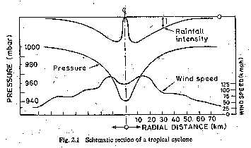
Fig.2.1 Schematic section of a tropical cyclone
They derive their energy from the latent heat of condensation of ocean water vapour and increase in size as they move on oceans. When they move on land the source of energy is cut off and the cyclone dissipates its energy very fast. Hence, the intensity of the storm decreases rapidly. Tropical cyclones cause heavy damage to life and property on their land path and intense rainfall and heavy floods in streams are its usual consequences. Tropical cyclones give moderate to excessive precipitation over very large areas, of the order of 10³ km² for several days.
Extratropical cyclone
These are cyclones formed in locations outside the tropical zone. Associated with a frontal system, they possess a strong counter-clockwise wind circulation in the northern hemisphere. The magnitude of precipitation and wind velocities are relatively lower than those of a tropical cyclone. However, the duration of precipitation is usually longer and the areal extent also is longer.
Anticyclones
These are regions of high Pressure, usually of large areal extent. The weather is usually calm at the centre. Anticyclones cause clockwise wind circulations in the northern hemisphere. Winds are of moderate speed, and at the outer edges, cloudy and precipitation conditions exist.
Convective Precipitation
In this type of precipitation a packet of air which is warmer than the surrounding air due to localised heating rises because of its lesser density. Air from cooler surroundings flows to take up its place thus setting up a convective cell. The warm air continues to rise, undergoes cooling and results in precipitation. Depending upon the moisture, thermal and other conditions light showers to thunderstorms can be expected in convective precipitation. Usually the areal extent of such rains is small, being limited to a diameter of about 10 km.
Orographic Precipitation
The moist air masses may get lifted-up to higher altitudes due to the presence of mountain barriers and consequently undergo cooling, condensation and precipitation. Such a precipitation is known as Orographic precipitation. Thus in mountain ranges, the windward slopes have heavy precipitation and the leeward slopes light rain fall.
CHARACTERISTIC OF PRECIPITATION ON INDIA
From the point of view of climate the Indian subcontinent can be considered to have two major seasons and two transitional periods as:
South-west monsoon (June-September)
Transition-1, post-monsoon (October-November)
Winter season (December-February)
Transition-11, Summer, (March-May)
South-West Monsoon (June-September)
The south-west monsoon (popularly known as the monsoon) is the principal rainy season of India when over 75% of the annual rainfall is received over a major portion of the country. Excepting the south-eastern part of the peninsula and Jammu and Kashmir, for the rest of the country the south-west monsoon is the principal source of rain with July as the rainiest month. The monsoon originates in the Indian ocean and heralds its appearance in the southern part of Kerala by the end of May. The onset of monsoon is accompanied by high south-westerly winds at speeds of 20-40 knots and low-pressure regions at the advancing edge. The monsoon winds advance across the country in two branches; Arabian sea branch and Bay of Bengal branch.
The former sets in at the extreme southern part of Kerala and the latter at Assam, almost simultaneously in the first week of June. The Bay branch first covers the north-eastern regions of the country and turns westwards to advance into Bihar and UP. The Arabian Sea branch moves northwards over Karnataka, Maharashtra and Gujarat. Both the branches reach Delhi around the same time by about the fourth week of June. A low-pressure region known as monsoon trough is formed between the two branches. The trough extends from the Bay of Bengal to Rajasthan and the precipitation pattern over the country is generally determined by its position. The monsoon winds increase from June to July and begin to weaken in September. The withdrawal of the monsoon, marked by a substantial rainfall activity starts in September in the northern part of the country. The onset and withdrawal of the monsoon at various parts of the country are shown in Fig. 2.2.
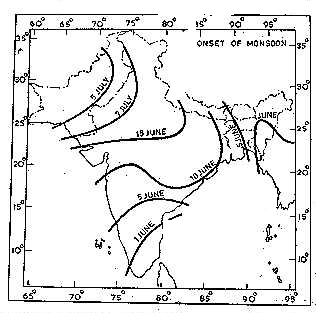
Fig.2.2 (a) Normal dates of onset of monsoon
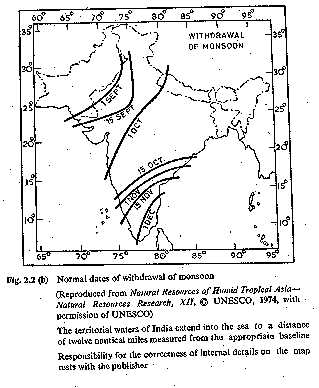
Fig.2.2 (b) Normal dates of withdrawal of monsoon
The monsoon is not a period of continuous rainfall. The weather is generally cloudy with frequent spells of rainfall. Heavy rainfall activity in various parts of the country owing to the passage of low pressure region is common. Depressions formed in the Bay of Bengal at a frequency of 2-3 per month move along the trough causing excessive precipitation of a 100-200 mm per day. Breaks of about a week in which the rainfall activity is the least is another feature of the monsoon. The south-west monsoon rainfall over the country is indicated in Fig. 2.3.
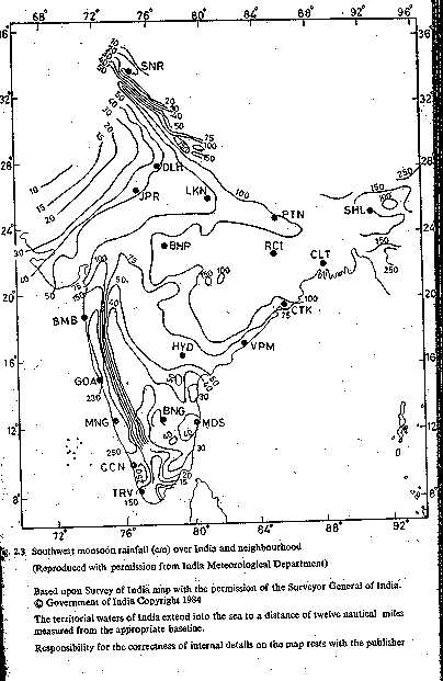
As seen from this figure the heavy rainfall areas are Assam and the north-eastern region with 200-400 cm; west coast and western ghats with 200-300 cm; West Bengal with 120-160 cm, UP, Haryana and the Punjab with 100-120 cm.
Post-Monsoon (October-November)
As the south-west monsoon retreats, low-pressure areas form in the Bay of Bengal and a north-easterly flow of air that picks UP moisture in the Bay of Bengal is formed. This air mass strikes the East Coast of the southern peninsula (Tamilnadu) and causes rainfall. Also, in this period, especially November, severe tropical cyclones form in the Bay of Bengal and Arabian Sea. The cyclones formed in the Bay of Bengal are about twice as many as in the Arabian Sea. These cyclones strike the coastal areas cause intense rainfall and heavy damage to life and property.
Winter Season (December-February)
By about mid-December, disturbances of extra tropical origin travel; wards across Afghanistan and Pakistan. Known as western disturbances, they cause moderate to heavy rain and snowfall (about 25 cm) in Himalayas and Jammu and Kashmir. Some light rainfall also occurs in northern plains. Low-pressure areas in the Bay of Bengal formed in the months cause 10-12 cm of rainfall in the southern parts of Tamilnadu.
Summer (Pre-monsoon) (March-May)
There is very little rainfall in India in this season. Convective cells cause some thunderstorms mainly in Kerala, West Bengal and Assam. Some cyclone activity, dominantly on the cast coast, also occurs.
Annual Rainfall
The annual rainfall over the country is shown in Fig. 2.4. Considerable areal variation exists for the annual rainfall in India with high rainfall the magnitude of 200 cm in Assam and north-eastern parts and the western ghats, and scanty rainfall in eastern Rajasthan and parts of Gujarat, Maharashtra and Karnataka. The average annual rainfall for the entire country is estimated as 119 cm. It is well known that there is considerable variation of annual rainfall in time at a place. The coefficient of variation,
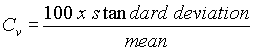
of the annual rainfall varies between 15 to 70, from place to place with an average value of about 30. Variability is least in regions of high rainfall and largest in regions of scanty rainfall. Gujarat, Haryana, the Punjab and Rajasthan have large variability of rainfall.
MEASUREMENT
Precipitation is expressed in terms of the depth to which rainfall water would stand on an area if all the rain were collected on it. Thus 1 cm of rainfall over a catchment area of 1 km² represents a volume of water equal to 104 m³. In the case of snowfall, an equivalent depth of water is used as the depth of precipitation. The precipitation is collected and measured in a raingauge. Terms such as pluviometer, ombrometer and hyetometer are also sometimes used to designate a raingauge. A raingauge essentially consists of a cylindrical-vessel assembly kept in the open to collect rain. The rainfall catch of the raingauge is affected by its exposure conditions. To enable the catch of raingauge to accurately represent the rainfall in the area surrounding the raingauge standard settings are adopted. For setting a raingauge the following considerations are important:
The ground must be level and in the open and the instrument must present a horizontal catch surface.
The gauge must be set as near the ground as possible to reduce wind effects but it must be sufficiently high to prevent splashing, flooding etc.
The instrument must be surrounded by an open fenced area of at least 5.5 m X 5.5 m. No object should be nearer to the instrument than 30 m or twice the height of the obstruction.
Raingauges can be broadly classified into two categories as non-recording raingauges and recording gauges.
Nonrecording Gauges
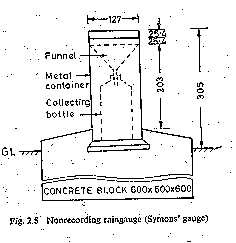
The nonrecording gauge extensively used in India is the Symons' gauge. It essentially consists of a circular collecting area of 12.7 cm (5.0 inch) diameter connected to a funnel. The rim of the collector is set in a horizontal plane at a height of 30.5 cm above the ground level. The funnel discharges the rainfall catch into a receiving vessel. The funnel and receiving vessel are housed in a metallic container. Figure 2.5 shows the details of the installation.
Water contained in the receiving vessel is measured by a suitably graduated measuring glass, with an accuracy up to 0.1 mm. Recently, the India Meteorological Department (IMD) has changed over to the use of fibreglass reinforced polyster raingauges, which is an improvement over the Symons' gauge. These come in different combinations of collector and bottle. The collector is in two sizes having areas of 200 and 100 cm² respectively. Indian Standard (IS : 5225-1969) gives details of these new raingauges.
For uniformity, the rainfall is measured every day at 8.30 AM (IST) and is recorded as the rainfall of that day. The receiving bottle normally does not hold more than 10 cm of rain and as such in the case of heavy rainfall the measurements must be done more frequently and entered. However, the last reading must be taken at 8.30 Am and the sum of the previous readings in the past 24 h entered as total of that day. Proper care' maintenance and inspection of raingauges, especially during dry weather to keep the instrument free from dust and dirt is very necessary. The details of installation of non-recording raingauges and measurement of rain are specified in Indian Standard (IS : 4986-1968). This raingauge can also be used to measure snowfall. When snow is expected, the funnel and receiving bottle are removed and the snow is allowed to collect in the outer metal container. The snow is then melted and the depth of resulting water measured. Antifreeze agents are some times used to facilitate melting of snow. In areas where considerable snowfall is expected, special snowgauges with shields (for minimizing the wind effect) and storage pipes (to collect snow over longer durations) are used.
Recording Gauges
Recording gauges produce a continuous Plot of rainfall against time and provide valuable data of intensity and duration of rainfall for hydrological analysis of storms. The following are some of the commonly used recording raingauges.
Tipping-Bucket Type
This is a 30.5 cm size raingauge adopted for use by the US Weather Bureau. The catch from the funnel falls onto one of a pair of small buckets. These buckets are so balanced that when 0.25 mm of rainfall collects in one bucket, it tips and brings the other one in position. The water from the tipped bucket is collected in a storage can. The tipping actuates an electrically driven pen to trace a record on clockwork-driven chart. The water collected in the storage can is measured at regular intervals to provide the total rainfall and also serve as a check. It may be noted that the record from the tipping bucket gives data on the intensity of rainfall. Further, the instrument is ideally suited for digitalizing of the output signal.
Weighing-Bucket Type
In this raingauge the catch from the funnel empties into a bucket mounted on a weighing scale. The weight of the bucket and its contents are recorded on a clockwork-driven chart. The clockwork mechanism has the capacity to run for as long as one week. This instrument gives a plot of the accumulated rainfall against the elapsed time, i.e. the mass curve of rainfall. In some instruments of this type the recording unit is so constructed that the pen reverses its direction at every preset value, say 7.5 cm (3 in.) so that a continuous plot of storm is obtained.
Natural-Syphon Type
This type of recording raingauge is also known as float-type gauge. Here the rainfall collected by a funnel-shaped collector is led into a float chamber causing a float to rise. As the float rises, a pen attached to the float through a lever system record the elevation of the float on a rotating drum driven by a clockwork mechanism. A syphon arrangement empties the float chamber when the float has reached a pre-set maximum level. This type of raingauge is adopted as the standard recording-type raingauge in India and its details are described in Indian Standard (IS : 5235-1969). A typical chart from this type of raingauge is shown in Figure 2.6.
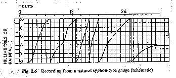
This chart shows a rainfall of 53.8 mm in 30 h. The vertical lines in the pen trace correspond to the sudden emptying of the float chamber by syphon action which resets the pen to zero level. It is obvious that the natural syphon-type recording raingauge gives a plot of the mass curve of rainfall.
Telemetering Raingauges
These raingauges are of the recording type and contain electronic transmit the data on rainfall to a base station both at regular inter on interrogation. The tipping-bucket type raingauge, being ideally suited is usually adopted for this purpose. Any of the other types of recording raingauges can also be used equally effectively. Telemetering gauges are utmost use in gathering rainfall data from mountainous and genera inaccessible places.
Radar Measurement of Rainfall
The meteorological radar is a powerful instrument for measuring the are extent, location and movement of rainstorms. Further, the amount rainfall over large areas can be determined through the radar with a go degree of accuracy. The radar emits a regular succession of pulses of electromagnetic radiation in a narrow beam. When raindrops intercept a radar beam, it has be shown that
 9; 9; 9; (2.1)
where Pr = average echo power, Z = radar-echo factor, r = distance target volume and C = a constant. Generally the factor Z is related to the intensity of rainfall as
![]() (2.2)
(2.2)
Where, a and b are coefficients and I = intensity or rainfall in mm/h. The values a and b for a given radar station have to be determined by calibration with the help of recording raingauges. A typical equation for Z is
Z = 200 I 1.60
Meteorological radars operate with wavelengths ranging from 3 to 10 cm, the common values being 5 and 10 cm. For observing details of heavy flood-producing rains, 10 cm radar is used while for light rain and snow a 5-em radar is used. The hydrological range of the radar is about 200 km. Thus a radar can be considered to be a remote-sensing super gauge covering an areal extent of as much as 100,000 km². Radar measurement is continuous in time and space. Present-day developments in the field include (i) On-line processing of radar data on a computer and (ii) Doppler-type radars for measuring the velocity and distribution of raindrops.
RAINGAUGE NETWORK
Since the catching area of a raingauge is very small compared to the areal extent of a storm, it is obvious that to get a representative picture of a storm over a catchment the number of raingauges should be as large as possible, i.e. the catchment area per gauge should be small. On the other hand, economic considerations to a large extent and other considerations, such as topography, accessibility, etc. to some extent restrict the number of gauges to be maintained. Hence one aims at an optimum density of gauges from which reasonably accurate information about the storms can be obtained. Towards this the World Meteorological Organisation (WMO) recommends the following densities.
In flat regions of temperate, Mediterranean and tropical zones:
ideal-1 station for 600-900 km², acceptable-1 station for 900-3000 km²;
In mountainous regions of temperate, Mediterranean and tropical zones: ideal-1 station for 100-250 km² acceptable-1 station for 250-1000 km²; and
In arid and polar zones: 1 station for 1500-10,000 km² depending on the feasibility.
Ten per cent of raingauge stations should be equipped with self-recording gauges to know the intensities of rainfall.
PREPARATION OF DATA
Before using the rainfall records of a station, it is necessary to first check the data for continuity and consistency. The continuity of a record may be broken with missing data due to many reasons such as damage or fault in a raingauge during a period. The missing data can be estimated by using the data of the neighboring stations. In these calculations the nor-mal rainfall is used as a standard of comparison. The normal rainfall is the average value of rainfall at a particular date, month or year over a specified 30-year period. The 30-year normals are recomputed every decade. Thus the term "normal annual precipitation" at station A means the average annual precipitation at A based on a specified 30 years of record.
Estimation of Missing Data
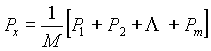
Given the annual precipitation values, P1, P2, P3, ... Pm at neighbouring M stations 1, 2, 3,..., M respectively, it is required to find the missing annual precipitation Px at a station X not included in the above M stations. Further, the normal annual precipitations NI, N2, ..., Ni... at each of the above (M + 1) stations including station X are known.
If the normal annual precipitations at various stations are within about 10% of the normal annual precipitation at station X, then a simple arithmetic average procedure is followed to estimate Px. Thus
 ; ; ; (2.4)
If the normal precipitation vary considerably, then Px is estimated by weighing the precipitation at the various stations by the ratios of normal annual precipitation. This method, known as the normal ratio method gives Px as
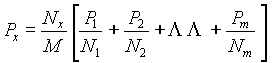 (2.5)
(2.5)
PRESENTATION OF RAINFALL DATA
A few commonly used methods of presentation of rainfall data which have been found to be useful in interpretation and analysis of such data are given below:
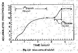
Mass Curve of Rainfall
The mass curve of rainfall is a plot of the accumulated precipitation against time, plotted in chronological order. Records of float type and weighing-bucket type gauges are of this form. A typical mass curve of rainfall at a station during a storm is shown in Fig. 2.8. Mass curves of rainfall are very useful in extracting the information on the duration and magnitude of a storm. Also, intensifies at various time intervals in a storm can be obtained by the slope of the curve. For non-recording raingauges, mass curves are prepared from a knowledge of the approximate beginning and end of a storm and by using the mass curves of adjacent recording gauge stations as a guide.
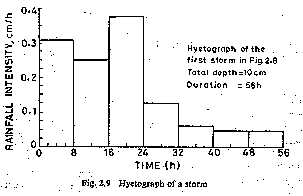
Hyetograph
A hyetograph is a plot of the intensity of rainfall against the time in The hyetograph is derived from the mass curve and is usually represented as a bar chart (Fig. 2.9). It is a very convenient way of represents characteristics of a storm and is particularly important in the development of a design storms to predict extreme floods. The area under a hyetograph represents the total precipitation received in that period. The time in used depends on the purpose; in urban-drainage problems small durations are used while in flood-flow computations in larger catchments the intervals are of about 6 h.
Point Rainfall
Point rainfall, also known as station rainfall refers to the rainfall data of a station. Depending upon the need, data can be listed as daily, wee monthly, seasonal or annual values for various periods. Graphically these data are represented as plots of magnitude vs chronological time in the form of a bar diagram. Such a plot, however, is not convenient for discerning trend in the rainfall as there will be considerable variations in the rainfall values leading to rapid changes in the plot. A moving-average plot, which the average value of precipitation of three or five consecutive time intervals is plotted at the mid-value of the time interval is useful smoothening out the variations and bringing out the trend.
MEAN PRECIPITATION OVER AN AREA
As indicated earlier, raingauges represent only point sampling of the areal distribution of a storm. In practice, however, hydrological analysis requires distribution of f the rainfall over an area, such as over a catchment. To convert the point rainfall values at various stations into an average value over a catchment the following three methods are in use:
• Arithmetical-mean method
• Thiessen-polygon method and
• Isohyetal method.
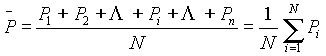
Arithmetical-Mean Method
When the rainfall measured at various stations in a catchment show little variation, the average precipitation over the catchment area is taken as the arithmetic mean of the station values. Thus if P1, P2,........., Pi......Pn are the rainfall values in a given period in N stations within a catchment, then the value of the mean precipitation ` P over the catchment by the arithmetic mean method is
 (2.7)
(2.7)
In practice, this method is used very rarely.
Thiessen-Mean Method
In this method the rainfall recorded at each station is given a weightage on the basis of an area closest to the station. The procedure of determining the weighing area is as follows: Consider a catchment area as in Fig. 2.10 containing three raingauge stations. There are three stations outside the catchment but in its neighbourhood. The catchment area is drawn to scale and the positions of the six stations marked on it. Stations 1 to 6 are joined to form a network of triangles. Perpendicular bisectors for, each of the sides of the triangle are drawn. These bisectors form a polygon around each station.

The boundary of the catchment, if it cuts the bisectors taken as the outer limit of the polygon. Thus for station 1, the bounding polygon is abcd. For station 2, kade is taken as the bounding polygon. These bounding polygons are called Thiessen polygons. The areas of these six Thiessen polygons are determined either with a planimeter or by using an overlay grid. If P1, P2, ..., P6, are the rainfall magnitudes recorded by the stations 1, 2, ..., 6 respectively, and A1, A2,.. .... A6, are the respective areas of the Thiessen polygons, then the average rainfall over the catchment ` P is given by
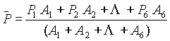
Thus in general for M stations,
 (2.8)
(2.8)
The ratio Ai /A is called the weightage factor for each station.
The Thiessen-polygon method of calculating the average precipitation over an area is superior to the arithmetic-average method as some weightage is given to the various stations on a rational basis. Further, the raingauge stations outside the catchment are also used effectively. Once the weightage factors are determined, the calculation of ` P is relatively easy for a fixed network of stations.
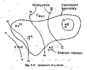
lsohyetal Method
An isohyetal is a line joining points of equal rainfall magnitude. In the isohyetal method, the catchment area is drawn to scale and the raingauge stations are marked. The recorded values for which area] average ` P is to be determined are then marked on the plot at appropriate stations. Neighbouring stations outside the catchment are also considered. The isohyets of various values are then drawn by considering point rainfalls as guides and interpolating between them by the eye (Figure 2.11). The procedure is similar to the drawing of elevation contours based on spot levels.
The area between two adjacent isohyets are then determined with planimeter. If the isohyets go out of catchment, the catchment boundary is used as the bounding line. The average value of the rainfall indicated by two isohyets is assumed to be acting over the inter-isohyet area. Thus P1, P2, .... Pn, are the values of isohyets and if a1, a2, ..., a n-1, are the inter-isohyet areas respectively, then the mean precipitation over the catchment of area A is given by
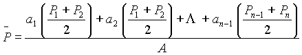 9; (2.9)
The isohyet method is superior to the other two methods especially when the stations are large in number.
DEPTH-AREA-DURATION RELATIONSHIPS
The areal distribution characteristics of a storm of given duration is reflected in its depth-area-relationship.
Depth-Area Relation
For a rainfall of a given duration, the average depth decreases with the area in an exponential fashion given by
&#` P = Po exp (- KAn) (2.10)
where ` P = average depth in cms over an area A km², Po= highest amount of rainfall in cm at the storm centre and K and n are constant for a given region. On the basis of 42 severe most storms in north India, Dhar and Bhattacharya (1975) have obtained the following values for K and n for storms of different duration.
| S.No. | Duration | K | n |
| 1 | Day | 0.0008526 | 0.6614 |
| 2 | Day | 0.0009877 | 0.6306 |
| 3 | Day | 0.001745 | 0.5961 |
Since it is very unlikely that the storm centre coincides over a raingauge station, the exact determination of Po is not possible. Hence in the analysis of large area storms the highest station rainfall is taken as the average depth over an area of 25 km².
Maximum Depth-Area-Duration Curves
In many hydrological studies involving estimation of severe floods, it is necessary to have information on the maximum amount of rainfall of various duration occurring over various sizes of areas. The development of relationship, between maximum depth-area-duration for a region is known as DAD analysis and forms an important aspect of hydro-meteorological study.
FREQUENCY OF POINT RAINFALL
In many hydraulic-engineering applications such as those concerned with floods, the probability of occurrence of a particular extreme rainfall, e.g. a 24-h maximum rainfall, will be of importance. Such information is obtained by the frequency analysis of the point-rainfall data. The rainfall at a place is a random hydrologic process and the rainfall data at a place when arranged in chronological order constitute a time series. One of the commonly used data series is the annual series composed of annual values such as annual rainfall. If the extreme values of a specified event occurring in each year is listed, it also constitutes an annual series. Thus for example, one may list the maximum 24-h rainfall occurring in a year at a station to prepare an annual series of 24-h maximum rainfall values. The probability of occurrence of an event in this series is studied by frequency analysis of this annual data series. A brief description of the terminology and a simple method of predicting the frequency of an event is described in this section and for details the reader is referred to standard works on probability and statistics. The analysis of annual series, even though described with rainfall as a reference is equally applicable to any other random hydrological process, e.g. stream flow.
First, it is necessary to correctly understand the terminology used in frequency analysis. The probability of occurrence of an event (e.g. rainfall) whose magnitude is equal to or in excess of a specified magnitude X is denoted by P. The recurrence interval (also known as return period) is defined as
T = 1/P
Plotting Position
The purpose of the frequency analysis of an annual series is to obtain a relation between the magnitude of the event and its probability of exceedence. The probability analysis may be made either by empirical or by analytical methods.
A simple empirical technique is to arrange the given annual extreme series in descending order of magnitude and to assign an order number m. Thus for the first entry m = 1, for the second entry m = 2 and so on till the last event for which m = N = Number of years of record. The probability P of an event equalled to or exceeded is given by the Weibull formula
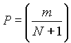 ; ; (2.14)
The recurrence interval T = 1/P = (N + 1)/m.
LOSSES FROM PRECIPITATION
Evaporation and transpiration form important links in the hydrologic cycle in which water is transferred to the atmosphere as water vapour. In engineering hydrology, runoff is the prime subject of study and evaporation and transpiration phases are treated as "losses". Evaporation from water bodies and soil masses together with the transpiration from vegetation is termed as evapotranspiration and is also known variously as water loss, total loss or total evaporation.
Before the rainfall reaches the outlet of a basin as runoff, certain demands of the catchment such as interception, depression storage and infiltration have to be met. If the precipitation not available for surface runoff is defined as "loss", then these processes are also "losses". In terms of groundwater the infiltration process is a "gain". Aspects of interception, depression storage and infiltration that are important from the point of view of engineering hydrology.
EVAPORATION PROCESS
Evaporation is the process in which a liquid changes to the gaseous state at the free surface, below the boiling point through the transfer of heat energy. Consider a body of water in a pond. The molecules of water are in constant motion with a wide range of instantaneous velocities. An addition of heat causes this range and average speed to increase. When they cross over the water surface. Similarly, the atmosphere in the immediate neighborhood or the water surface contains water molecules within the water vapour in motion and some of them penetrate the water surface. The net escape of water molecules from the liquid state to the gaseous state constitute evaporation. Evaporation is a cooling process in that the latent heat of vaporization (at about 585 cal/g of evaporated water) must be provided by the water. The rate of evaporation is dependent on
• Vapour pressure at the water surface
• Air and water temperatures,
• Wind speed,
• Atmospheric pressure,
• Quality of water and
• Size of the water body.
Vapour Pressure
The rate of evaporation is proportional to the difference between the saturation vapour pressure at the water temperature, ew and the actural vapour pressure in the air, ea. Thus EL = C (ew -ea) #9; #9; (3.1)
Where, EL = rate of evaporation (mm/day) and C = a constant; ew and ea, are in mm of mercury. This Equation is known as Dalton's law of evaporation after John Dalton (1802) who first recognised this law. Evaporation continue till ew = ea. If ew > ea, condensation takes place.
Temperature
Other factors remaining same, the rate of evaporation increases with an increase in the water temperature. Regarding air temperature, although there is a general increase in the evaporation rate with increasing temperature, a high correlation between evaporation rate and air temperature does not exist. Thus for the same mean monthly temperature it is possible to have evaporation to different degrees in a lake in different months.
Wind
Wind aids in removing the evaporated water vapour from the zone of evaporation and consequently creates greater scope for evaporation. However, if the wind velocity is large enough to remove all the evaporated water vapour, any further increase in wind velocity does not influence the evaporation. Thus the rate of evaporation increases with the wind-speed up to a critical speed beyond which any further increase in the wind speed has no influence on the evaporation rate. This critical wind-speed value is a function of the size of the water surface. For large water bodies, high-speed turbulent winds are needed to cause maximum rate of evaporation.
Atmospheric Pressure
Other factors remaining same, a decrease in the barometric pressure, as in high altitudes, increases evaporation.
Soluble Salts
When a solute is dissolved in water, the vapour pressure of the solution is less than that of pure water and hence causes reduction in the rate of evaporation. The per cent reduction in evaporation approximately corresponds to the percentage increase in the specific gravity. Thus, for example, under identical conditions evaporation from sea water is about 2-3% less than that from fresh water.
Heat Storage in Water Bodies
Deep water bodies have more heat storage than shallow ones. A deep lake may store radiation energy received in summer and release it in winter causing less evaporation in summer and more evaporation in winter com-pared to a shallow lake exposed to a similar situation. However, the effect of heat storage is essentially to change the seasonal evaporation rates and the annual evaporation rate is seldom affected.
EVAPORIMETERS
Estimation of evaporation is of utmost importance in many hydrologic problems associated with planning and operation of reservoirs and irrigation systems. In and zones, this estimation is particularly important to conserve the scarce water resources. However, the exact measurement of evaporation from a large body of water is indeed one of the most difficult tasks. The amount of water evaporated from a water surface is estimated by the following methods:
• Using evaporimeter data,
• Empirical evaporation equations and
• Analytical methods.
Types of Evaporimeters
Evaporimeters are water-containing pans which are exposed to the atmosphere and the loss of water by evaporation measured in them at regular intervals. Meteorological data, such as humidity, wind movement, air and water temperatures and precipitation are also noted along with evaporation measurement.
Many types of evaporimeters are in use and a few commonly used pans are :
Class A Evaporation Pan
It is a standard pan of 1210 mm diameter and 255 mm depth used by theUS Weather Bureau and is known as Class A Land Pan. The depth of water is maintained between 18 em and 20 em (Fig. 3.1). The pan is normally made of unpainted galvanised iron sheet. Monel metal is used where corrosion is a problem. The pan is placed on a wooden platform of 15 cm height above the ground to allow free circulation of air below the pan. Evaporation measurements are made by measuring the depth of water with a hook gauge in a stilling well.
ISI Standard Pan
This pan evaporimeter specified by IS:5973-1970, also known as modified Class A Pan, consists of a pan 1220 mm in diameter with 255 mm of depth. The pan is made of copper sheet of 0.9 mm thickness, tinned inside and painted white outside (Fig. 3.2). A fixed point gauge indicates the level of water. A calibrated cylindrical measure is used to add or remove water maintaining the water level in the pan to a fixed mark. The top of the pan is covered fully with a hexagonal wire netting of galvanized iron to protect the water in the pan from birds. Further, the presence of a wire mesh makes the water temperature more uniform during day and night.
The evaporation from this pan is found to be less by about 14% compared to that from unscreened pan. The pan is placed over a square wooden platform of 1225 mm width and 100 mm height to enable circulation of air underneath the pan.
Colorado Sunken Pan
This pan, 920 mm square and 460 mm deep is made up of unpainted galvanised iron sheet and buried into the ground within 100 mm of the top (Fig. 3.3). The chief advantage of the sunken pan is that radiation and aerodynamic characteristics are similar to those of a lake. However, it has the disadvantages like difficult to detect leaks, extra care is needed to keep the surrounding area free from tall grass, dust etc. and expensive to install.
US Geological Survey Floating Pan
With a view to simulate the characteristics of a large body of water, this square pan (900 mm side and 450 mm depth) supported by drum floats in the middle of a raft (4.25 m X 4.87 m) is set afloat in a lake. The water level in the pan is kept at the same level as the lake leaving a rim of 75 mm. Diagonal baffles provided in the pan reduce the surging in the pan due to wave action. Its high cost of installation and maintenance together with the difficulty involved in performing measurements are its main disadvantages.
Pan Coefficient, Cp
Evaporation pans are not exact models of large reservoirs and have the following principal drawbacks:
They differ in the heat-storing capacity and heat transfer from the sides and bottom. The sunken pan and floating pan aim to reduce this deficiency. As a result of this factor the evaporation from a pan depends to a certain extent on its size. While a pan of 3 m diameter is known to give a value which is about the same as from a neighbouring large lake, a pan of size 1.0 m diameter indicates about 20% excess evaporation than that of the 3 m diameter pan.
The height of the rim in an evaporation pan affects the wind action over the surface. Also, it casts a shadow of variable magnitude over the water surface.
The heat-transfer characteristics of the pan material is different from that of the reservoir.
In view of the above, the evaporation observed from a pan has to be corrected to get the evaporation from a lake under similar climatic and exposure conditions. Thus a coefficient is introduced as
Lake evaporation = Cp X pan evaporation
in which Cp = pan coefficient. The values of Cp in use for different pan are given in Table 3. I.
TABLE 3.1 VALUES OF PAN COEFFICIFNT Cp
S. No. |
Type of pan | Average value | Range |
| 1 | Class A Land Pan | 0.70 | 0.60-0.80 |
| 2 | ISI Pan (modified Class A) | 0.80 | 0.65-1.10 |
| 3 | Colorado Sunken Pan | 0.78 | 0.75-0.86 |
| 4 | USGS Floating Pan | 0.80 | 0.70-0.82 |
Evaporation Stations
It is usual to install evaporation pans in such locations where other meteorological data are also simultaneously collected. The WMO recommend the minimum network of evaporimeter stations as below:
• Arid zones-One station for every 30,000 km²,
• Humid temperate climates-one station for every 50,000 km², and
• Cold regions-One station for every 100,000 km².
Currently India has about 200 pan-evaporimeter stations maintained by the India Meteorological Department.
TRANSPIRATION
Transpiration is the process by which water leaves the body of a living plant and reach the atmosphere as water vapour. The water is taken up by the plant-root system and escapes through the leaves. The important factors affecting transpiration are: atmospheric vapour pressure, temperature, wind, light intensity and characteristics of the plant, such as the root and leaf systems. For a given plant, factors that affect the free-water evaporation also affect transpiration. However, a major difference
exists between transpiration and evaporation. Transpiration is essentially confined to daylight hours and the rate of transpiration depends upon the growth periods of the plant. Evaporation, on the other hand, continues all through the day and night although the rates are different.
EVAPOTRANSPIRATION
While transpiration takes place, the land area in which plants stand also lose moisture by the evaporation of water from soil and water bodies. In hydrology and irrigation practice, it is found that evaporation and transpiration processes can be considered advantageously under one head as evapotranspiration. The term consumptive use is also used to denote this loss by evapotranspiration. For a given set of atmospheric conditions, evapotranspiration obviously depends on the availability of water. If sufficient moisture is always available to completely meet the needs of vegetation fully covering the area, the resulting evapotranspiration is called potential evapotranspiration (PET). Potential evapotranspiration no longer critically depends on soil and plant factors but depends essentially on climatic factors. The real evapotranspiration occurring in a specific situation is called actual evapotranspiration (AET). It is necessary to introduce at this stage two terms: field capacity and permanent wilting point. Field capacity is the maximum quantity of water that the soil can retain against the force of gravity. Any higher moisture input to a soil at field capacity simply drains away. Permanent wilting Point is the Moisture Content of a soil at which the moisture is no longer available in sufficient quantity to sustain the plants. At this stage, even though the soil contains some moisture, it will be so held by the soil grains that the roots of the plants are not able to extract it in sufficient quantities to sustain the plants and consequently the plants wilt. The field capacity and permanent wilting point depend upon the soil characteristics. The difference between these two moisture contents is called available water, the moisture available for plant growth. If the water supply to the plant is adequate, soil moisture will be at the field capacity and AET will be equal to PET. If the water supply is less than PET, the soil dries out and the ratio AET/PET would then be less than unity. The decrease of the ratio AET/PET with available moisture depends upon the type of soil and rate of drying. Generally, for clayey soils, AET/PET» 1.0 for nearly 50% drop in the available moisture. As can be expected, when the soil moisture reaches the permanent wilting point, the AET reduces to zero (Fig.3.5). For a catchment in a given period of time, the hydrologic budget can be written as
P – Rs – Go - Eact = D S ; ; (3.12)

Where, P = precipitation, Rs = surface runoff, Go = subsurface outflow, Eact = actual evapotranspiration (AET) and D S = change in the moisture storage. This water budgeting can be used to calculate Eact by knowing or estimating other elements of above equation. The sum of Rs and Go can be taken as the stream flow R at the basin outlet without much error.
Except in a few specialised studies, all applied studies in hydrology use PET for various estimation purposes. It is generally agreed that PET is a good approximation for lake evaporation.
MEASUREMENT OF EVAPOTRANSPIRATION
The measurement of evapotranspiration for a given vegetation type can be carried out in two ways: either by using lysimeters or by the use of field plots.
Lysimeters
A lysimeter is a special watertight tank containing a block of soil and set in a field of growing plants. The plants grown in the lysimeter are the same as in the surrounding field. Evapotranspiration is estimated in terms of the amount of water required to maintain constant moisture conditions within the tank measured either volumetrically or gravimetrically through an arrangement made in the lysimeter. Lysimeters should be designed to accurately reproduce the soil conditions, moisture content, type and size of the vegetation of the surrounding area. They should be so hurried that the soil is at the same level inside and outside the container. Lysimeter studies are time-consuming and expensive.
Field Plots
In special plots all the elements of the water budget in a known interval of time are measured and the evapotranspiration determined as
Evapotranspiration = [precipitation + irrigation input - runoff - increase in soil storage
- groundwater loss]
Measurements are usually confined to precipitation, irrigation input, surface runoff and soil moisture. Groundwater loss due to deep percolation is difficult to measure and can be minimised by keeping the moisture condition of the plot at the field capacity. This method provides fairly reliable results.
POTENTIAL EVAPOTRANSPIRATION OVER INDIA
Using Penman's equation and the available climatalogical data, PET estimated for the country has been made. The mean annual PET (in cm) over various parts of the country is shown in the form of isopleths - the lines on a map through places having equal depths of evapotranspiration. It is seen that the annual PET ranges from 140 to 180 cm over most parts of the country. The annual PET is highest at Rajkot, Gujarat with a value or 214.5 cm. Extreme south-east of Tamil Nadu also show high average values greater than 180 cm. The highest PET for southern peninsula is at Tiruchirapalli, Tamil Nadu with a value of 209 cm. The variation of monthly PET at stations located in various climatic zones in the country.
INITIAL LOSS
In the precipitation reaching the surface of a catchment the major abstraction is from the infiltration process. However, two other processes, though small in magnitude, operate to reduce the water volume available for runoff and thus act as abstractions. These are the interception process and the depression storage, and together they are called initial loss. This abstraction represents the quantity of storage that must be satisfied before overland runoff begins. The following two sections deal with these two processes briefly.
INTERCEPTION
When it rains over a catchment not all the precipitation falls directly onto the ground. Before it reaches the ground, a part of it may be caught by the vegetation and subsequently evaporated. The volume of water so caught is called interception. The intercepted precipitation may follow one of the three possible routes:
It may be retained by the vegetation as surface storage and returned to the atmosphere by evaporation; a process termed interception loss;
It can drip off the plant leaves to join the ground surface or. the surface flow; this is known as throughfall; and
The rainwater may run along the leaves and branches and down the stem to reach the ground surface. This part is called stemflow.
Interception loss is solely due to evaporation and does not include transpiration, through fall or stemfiow.
The amount of water intercepted in a given area is extremely difficult to measure. It depends on the species composition density and also on the storm characteristics. It is estimated that of the total rainfall in an area during a plant-growing season the interception loss is about 10 to 20%.
Interception is satisfied during the first part of a storm and if an area experiences a large number of small storms, the annual interception loss due to forests in such cases will be high, amounting to greater than 25% of the annual precipitation. Quantitatively, the variation of interception loss with the rainfall magnitude per storm for small storms is as shown in Fig. 3.7. It is seen that the interception loss is large for a small rainfall and levels off to a constant value for larger storms.
For a given storm, the interception loss is estimated as
Ii = Si + Ki Et ; ; (3.18)
Where Ii = interception loss in mm, Si = interception storage whose value varies from 0.25 to 1.25 mm depending on the nature of vegetation, Ki = ratio of vegetal surface area to its projected area, E = evaporation rate in mm/h during the precipitation and t = duration of rainfall in hours.
It is found that coniferous trees have more interception loss deciduous ones. Also, dense grasses have nearly same interception losses as full grown trees and can account for nearly 20% of the total rainfall in a season. Agricultural crops in their growing season also contribute high interception losses. In view of these the interception process has a very significant impact on the ecology of the area related to silvicultural aspects and in the water balance of a region. However, in hydrological studies dealing with floods interception loss is rarely significant and is not separately considered, The common practice is to allow a lump sum value as the initial loss to be deducted from the initial period of the storm.
DEPRESSION STORAGE
When the precipitation of a storm reaches the ground, it must first fill up all depressions before it can flow over the surface. The volume of water trapped in these depressions is called depression storage. This amount is eventually lost to runoff through processes of infiltration and evaporation and thus form a part of the initial loss. Depression storage depends on a vast number of factors the chief of which are :
• The type of soil,
• The condition of the surface reflecting the amount and nature of depression,
• The slope of the catchment and
• The antecedent precipitation, as a measure of the soil moisture. Obviously,
general expressions for quantitative estimation of this loss are not available.
Qualitatively, it has been found that antecedent precipitation has a very
pronounced effect on decreasing the loss to runoff in a storm due to depression.
Values of 0.50 cm in sand, 0.4 cm in loam and 0.25 cm in clay can be taken as
representatives for depression-storage loss during intensive storms.
INFILTRATION PROCESS
It is well-known that when water is applied to the surface of a soil, a part of it seeps into the soil. This movement of water through the soil surface is known as infiltration and plays a very significant role in the runoff process by affecting the timing, distribution and magnitude of the surface runoff. Further, infiltration is the primary step in the natural groundwater recharge.
Infiltration is the flow of water into the ground through the soil surface and the process can be easily understood through a simple analogy. Consider a small container covered with wire gauze as in Fig. 3.8. If water is poured over the gauze, a part of it will go tainer and a part overflows. Further, the container can hold only a fixed quantity and when it is full no more flow into the container can take place. This analogy, though a highly simplified one, underscores two important aspects, viz., the maximum rate at which the ground can absorb water, the infiltration capacity and the volume of water that it can hold, the field capacity.
Since the infiltered water may contribute to groundwater discharge in addition to increasing the soil moisture, the process can be schematically modelled as in Fig. 3.9(a) and (b). This figure considers two situations, viz. low-intensity rainfall and high intensity rainfall, and is self explanatory.
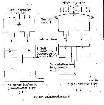
Fig. 3.9 An infiltration model
INFILTRATION CAPACITY
The maximum rate at which a given soil at a given time can absorb water is defined as the infiltration capacity. It is designated as fc and is expressed in units of cm/h. The actual rate of infiltration f can be expressed as
f = fc when i > fc ; ; (3.19)
f = i when i < fc
where i = intensity of rainfall. The infiltration capacity of a soil is high at the beginning of a storm and has an exponential decay as the time elapses. The infiltration process is affected by a large number of factor and a few important ones affecting fc are described below.
Characteristics of Soil
The type of soil, viz. sand, silt or clay, its texture, structure, permeability and under drainage are the important characteristics under this category. A loose, permeable, sandy soil will have a larger infiltration capacity than a tight, clayey soil. A soil with good under drainage, i.e. the facility to transmit the infiltered water downward to a groundwater storage would obviously have a higher infiltration capacity. When the soils occur in layers, the transmission capacity of the layers determine the overall infiltration rate. Also a dry soil can absorb more water than one whose pores are already full. The land use has a significant influence on fc. For example, a forest soil rich in organic matter will have a much higher value of fc under identical conditions than the same soil in an urban area where it is subjected to compaction.
Surface of Entry
At the soil surface, the impact of raindrops causes the fines in the soils to be displaced and these in turn can clog the pore spaces in the upper layers. This is an important factor affecting the infiltration capacity. Thus a surface covered by grass and other vegetation which can reduce this process has a pronounced influence on the value of fc.
Fluid Characteristics
Water infiltrating into the soil will have many impurities, both in solution and in suspension. The turbidity of the water, especially the clay and colloid content is an important factor as such suspended particles block the fine pores in the soil and reduce its infiltration capacity. The temperature of the water is a factor in the sense that it affects the viscosity of the water which in turn affects the infiltration rate. Contamination of the water by dissolved salts can affect the soil structure and in turn affect the infiltration rate.
MEASUREMENT OF INFILTRATION
Information about the infiltration characteristics of the soil at a given location can be obtained by conducting controlled experiments on small areas. The experimental set-up is called an infiltrometer. There are two kinds of infiltrometers :
Flooding-type infiltrometer
Rainfall simulator.
Flooding-Type lnfiltrometer
This is a simple instrument consisting essentially of a metal cylinder, 30 cm diameter and 60 cm long, open at both ends. This cylinder is driven into the ground to a depth of 50 cm (Fig.3.10). Water is poured into the top part to a depth of 5 cm and a pointer is set to mark the water level. As infiltration proceeds, The volume is made up by adding water from a burette to keep the water level at the tip of the pointer. Knowing the volume of water added at different time intervals, the plot of the infiltration capacity vs lime is obtained. The experiments are continued till a uniform rate of infiltration is obtained and this may take 2-3 h. The surface of the soil is usually protected by a perforated disk to prevent formation capacity vs lime is obtained. The experiments re continued till a uniform rate of infiltration is obtained and this may take 2-3 h.
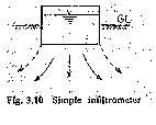
Fig.3.10 Simple infiltrometer
The surface of the soil is usually protected by a perforated disk to prevent formation of turbidity and its settling on the soil surface.
A major objection to the simple infiltrometer as above is that the infiltered water spreads at the outlet from the tube (as shown by dotted lines in Fig. 3.10) and as such the tube area is not representative of the area in which infiltration takes place. To overcome this a ring infiltrometer consisting of a set of two concentric rings (Fig.3.11) is used. In this two rings are inserted into the ground and water is maintained on the soil surface, in both the rings, to a common fixed level. The outer ring provides a water jacket to the infiltering water of the inner ring and hence prevents the spreading out of the infiltering water of the inner tube. The measurements of water volume is done on the inner ring only.
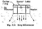
Fig.3.11 Ring infiltrameter
The main disadvantages of flooding-type infiltrometer are :
• Raindrop-impact effect is not simulated;
• Driving of the tube or rings disturbs the soil structure;
• Results of the infiltrometer depend to some extent on their size with the larger
meters giving less rates than the smaller ones; this is due to the border effect.
Rainfall Simulator
In this a small plot of land, of about 2 m X 4 m size, is provided with a size of nozzles on the longer side with arrangements to collect and measure the surface runoff rate. The specially designed nozzles produce raindrops falling from a height of 2 m and are capable of producing various intensities of rainfall. Experiments are conducted under controlled conditions with various combinations of intensities and durations and the surface runoff is measured in each case. Using the water-budget equation involving the volume of rainfall, infiltration and runoff, the infiltration rate and its variation with time is calculated. If the rainfall intensity is higher than the infiltration rate, infiltration-capacity values are obtained.
Rainfall simulator type infiltrometers given lower values than flooding type infiltrometers. This is due to the effect of the rainfall impact and turbidity of the surface water present in the former.
INFILTRATION-CAPACITY VALUES
The typical variation of the infiltration capacity for two soils and for two initial conditions is shown in Fig. 3.12. It is clear from the figure that the infiltration capacity for a given soil decreases with time from the start of rainfall; it decreases with the degree of saturation and depends upon the type of soil. Horton (1930) expressed the decay of the infiltration capacity with time as
![]() (3.20)
(3.20)
Where,
fct = infiltration capacity at any time t from start of the rainfall
fco = initial infiltration capacity at t = 0
fcf = final steady state value
td = duration of the rainfall and
Kh = constant depending upon the soil characteristics and vegetation cover.
The difficulty of finding the variation of the three parameters fco, fcf and Kh with soil characteristics and antecedent moisture conditions precludes the general use of Eq. (3.20).
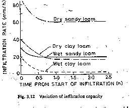
Fig. 3.12 Variation of infiltration capacity
It is apparent that infiltration-capacity values of soils are subjected to wide variations depending upon a large number of factors. Typically, a bare, sandy area will have fc » 1.2 cm/h and a bare, clay soil will have fs » 0.15 cm/h. A good grass cover or vegetation cover increases these values by as much as 10 times.
INFILTRATION INDICES
In hydrological calculations involving floods it is found convenient to use a constant value of infiltration rate for the duration of the storm. The average infiltration rate is called infiltration index and two types of indices are in common use.
The F index is the average rainfall above which the rainfall volume is equal to the runoff volume. The F index is derived from the rainfall hyetograph with the knowledge of the resulting runoff volume. The initial loss is also considered as infiltration. The F value is found by treating it
as a constant infiltration capacity. If the rainfall intensity is less than 0, then the infiltration rate is equal to the rainfall intensity; however, if the rainfall intensity is larger than F the difference between rainfall and infiltration in an interval of time represents the runoff volume (Fig. 3.13). The amount of rainfall in excess of the F index is called rainfall excess. The F index thus accounts for the total abstraction and enables runoff magnitudes to be estimated for a given rainfall hyetograph.
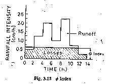
Fig.3.13 f Index
STREAMFLOW MEASUREMENT
Streamflow representing the runoff phase of the hydrologic cycle is the most important basic data for hydrologic studies. It was seen in the previous chapters that precipitation, evaporation and evapotranspiration are all difficult to measure exactly and the presently, adopted methods have severe limitations. In contrast the measurement of streamflow is amenable to fairly accurate assessment. Interestingly, streamflow is the only part of the hydrologic cycle that can be measured accurately.
A stream can be defined as a flow channel into which the surface runoff from a specified basin drains. Generally, there is considerable exchange of water between a stream and the underground water. Streamflow is measured in units of discharge (m³/s) occurring at a specified time and constitutes historical data. The measurement of discharge in a stream forms an important branch of Hydrometry, the science and practice of water measurement. This chapter deals with only the salient streamflow measurement techniques to provide an appreciation of this important aspect of engineering hydrology.
Streamflow measurement techniques can be broadly classified into two categories as (i) direct determination and (ii) indirect determination.
1. Direct determination of stream discharge:
(a) Area-velocity methods,
(b) Dilution techniques,
(c) Electromagnetic method, and
(d) Ultrasonic method.
2. Indirect determination of stream flow:
(a) Hydraulic structures, such as weirs, flumes and gated structures
(b) Slope-area method.
Barring a few exceptional cases, continuous measurement of stream discharge is very difficult to obtain. As a rule, direct measurement of discharge is a very time-consuming and costly procedure. Hence, a two step procedure is followed. First, the discharge in a given stream is related to the elevation of the water surface (stage) through a series of careful measurements. In the next step the stage of the steam is observed routinely in a relatively inexpensive manner and the discharge is estimated by using the previously determined stage-discharge relationship. The observation of the stage is easy, inexpensive, and if desired, continuous readings can also be obtained. This method of discharge determination of streams is adopted universally.
MEASUREMENT OF STAGE
The stage of a river is defined as its water-surface elevation measured above a datum. This datum can be the mean-sea level (MSL) or an arbitrary datum connected independently to the MSL.
Staff Gauge
The simplest of stage measurements are made by noting the water surface in contact with a fixed graduated staff. The staff is made of a durable material with a low coefficient of expansion with respect both temperature and moisture. It is fixed rigidly to a structure, such an abutment, pier, wall, etc. The staff may be vertical or inclined with clearly and accurately graduated permanent markings. The markings a distinctive, easy to read from a distance and are similar to those or surveying staff. Sometimes, it may not be possible to read the entire range of water-surface elevations of a stream by a single gauge and in such cases the gauge is built in sections at different locations. Such gauges called sectional gauges (Fig. 4.1). When installing sectional gauges, must be taken to provide an overlap between various gauges and to all the sections to the same common datum.
Wire Gauge
If is a gauge used to measure the water-surface elevation from above the surface such as from a bridge or similar structure. In this a weight is lowered by a reel to touch the water surface. A mechanical counter measures the rotation of the wheel which is proportional to the length of
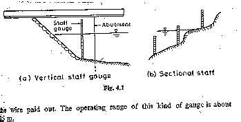
Fig.4.1 (a) Vertical staff gauge (b) Sectional staff
the wire paid out. The operating range of this kind of gauge is about 25 m.
Automatic Stage Recorders
The staff gauge and wire gauge described earlier are manual gauges. While they are simple and inexpensive, they have to be read at frequent intervals to define the variation of stage with time accurately. Automatic stage recorders overcome this basic objection of manual staff gauges and find considerable use in stream-flow measurement practice. Two typical automatic stage recorders are described below.
Float-Gauge Recorder
The Float-operated stage recorder is the most common type of automatic stage recorder in use. In this a float operating in a stifling well is balanced by means of a counterweight over the pulley of a recorder. Displacement of the float due to the rising or lowering of the water-surface elevation causes an angular displacement of the pulley and hence of the input shaft of the recorder. Mechanical linkages convert this angular displacement to the linear displacement of a pen to record over a drum driven by clockwork. The pen traverse is continuous with automatic reversing when it reaches the full width of the chart. A clockwork mechanism runs the recorder for a day, week or fortnight and provides a continuous plot of stage vs time. A good instrument will have a large-size float and least friction. Improvements over this basic analogue model consists of models that give digital signals recorded on a punched tape, magnetic tape or transmit directly onto a central data-processing centre.
To protect the float from debris and to reduce the water surface wave effects on the recording, stifling wells are provided in all float-type stage-recorder installations. Figure 4.2 shows a typical stifling well installation. Note the intake pipes that communicate with the river and flushing arrangement to flush these intake pipes off the sediment and debris occasionally. The water-stage recorder has to be located above the highest water level expected in the stream to prevent it from getting inundated
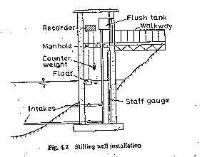
Fig. 4.2 Stilling well installation
during floods. Further, the instrument must be properly housed in a suitable enclosure to protect it from weather elements and vandalism. On account of these, the water-stage-recorder installations prove to costly in most instances. A water-depth recorder is shown in Fig.4.3 (Plate 1).
Bubble Gauge
In this gauge compressed air or gas is made to bleed out at a very small rate through an outlet Placed at the bottom of the river [fig.4.4, 4.5(plate 1) and 4.6 (Plate 11)]. A pressure gauge measures the gas pressure which in turn is equal to the water column above the outlet. A small change in the water-surface elevation is felt as a change in pressure from the present value at the pressure gauge and this in turn is adjusted by a servo-mechanism to bring the gas to bleed at the original rate under the new head. The pressure gauge reads the new water depth which transmitted to a recorder.
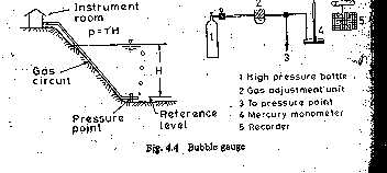
Fig.4.4 Bubble Gauge
The bubble gauge has certain specific advantages over a float operated water stage recorder and these can be listed as under :
• There is no need for costly stifling wells;
• A large change in the stage, as much as 30 m, can be measured;
• The recorder assembly can be quite far away from the sensing point; and
• Due to constant bleeding action there is less likelihood of the inlet getting
blocked or choked.
Stage Data
The stage data is often presented in the form of a plot of stage against chronological time (Figure 4.7) known as stage hydrograph. In addition to its use in the determination of stream discharge, stage data itself is of importance in flood warning and flood-protection works. Reliable long-term stage data corresponding to peak floods can be analysed statistically to estimate the design peak river stages for use in the design of hydraulic structures, such as bridges, weirs, etc. Historic flood stages are invaluable in the indirect estimation of corresponding flood discharges. In view of these multifarious uses, the river stage forms an important hydrologic parameter chosen for regular observation and recording.
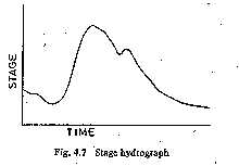
Fig. 4.7 Stage hydrograph
MEASUREMENT OF VELOCITY
The measurement of velocity is an important aspect of many direct stream-flow measurement techniques. A mechanical device, called current meter, consisting essentially of a rotating element is probably the most commonly used instrument for accurate determination of the stream-velocity field. Approximate stream velocities can be determined by floats.
Current Meters
The most commonly used instrument in hydrometry to measure the velocity at a point in the flow cross-section is the current meter. It consists essentially of a rotating element which rotates due to the reaction of the stream current with an angular velocity proportional to the stream velocity. Historically, Robert Hooke (1663) invented a propeller-type current meter to measure the distance traversed by a ship. The present-day cup-type instrument and the electrical make-and-break mechanism were invented by Henry in 1868. There are two main types of current meters.
Vertical-axis meters, and
Horizontal-axis meters.
Vertical-Axis Meters
These instruments consist of a series of conical cups mounted around a vertical axis [Figs. 4.8 and 4.9 (Plate 111)]. The cups rotate in a horizontal plane and a cam attached to the vertical axial spindle records generated signals proportional to the revolutions of the cup assembly. The Price current meter and Gurley current meter are typical instruments under this category. The normal range of velocities is from 0.15 to 0.40 m/s. The accuracy of these instruments is about 1.50% at the threshold value and improves to about 0.30% at speeds in excess of 1.0 m/s.
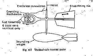
Fig. 4.8 Vertical-axis current meter
Vertical-axis instruments have the disadvantage that they cannot be used where there are appreciable vertical components of velocities. For example, the instrument shows a positive velocity when it is lifted vertically in still water.
Horizontal-Axis Meters
These meters consist of a propeller mounted at the end of a horizontal shaft [Fig. 4.10 (Plate 111) and 4.11]. These come in a wide variety of sizes with propeller diameters in the range 6 to 12 cm and can register velocities in the range of 0.15 to 4.0 m/s. Ott-, Neyrtec= [Fig. 4.12 (Plate IV)] and Watt-type meters are typical instruments under this kind.
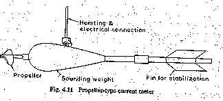
Fig. 4.11 Propeller,type current meter
These meters are fairly rugged and are not affected by oblique flows of as much as 15°. The accuracy of the instrument is about 1% at the threshold value and is about 0.25% at a velocity of 0.3 m/s and above.
A current meter is so designed that its rotation speed varies linearly with the stream velocity v at the location of the instrument. A typical relationship is
v = a Ns+ b (4.1)
where v = stream velocity at the instrument location in m/s,
Ns = revolutions per second of the meter and
a, b = constants of the meter. Typical values of a and b for a standard size 12.5 cm dia Price meter (cup-type) is a = 0.65 and b = 0.03. Smaller meters of 5 cm. diameter cup assembly called pigmy meters run faster and are useful in measuring small velocities. The values of the meter constants for them are of the order of a = 0.30 and b = 0.003. Further, each instrument has a threshold velocity below which Eq. (4.1) is not applicable. The instruments have a provision to count the number of revolutions in a known interval of time. This is usually accomplished by the making and breaking of an electric
circuit either mechanically or electro-magnetically at each revolution of the shaft. In older model instruments the breaking of the circuit would be counted through an audible sharp signal ("tick") heard on a headphone. The revolutions per second is calculated by counting the number of such signals in a known interval of time, usually about 100 s. Present-day models employ electromagnetic counters with digital or analogue displays.
Calibration
The relation between the stream velocity and revolutions per second of the meter as in Eq. (4.1) is called the calibration equation. The calibration equation is unique to each instrument and is determined by towing the instrument in a special tank. A towing tank is a long channel containing still water with arrangements for moving a carriage longitudinally over its surface at constant speed. The instrument to be calibrated is mounted on the carriage with the rotating element immersed to a specified depth in the water body in the tank. The carriage is then towed at a predetermined constant speed (v) and the corresponding average value of revolutions per second (Ns) of the instruments determined. This experiment is repeated over the complete range of velocities and a best-fit linear relation in the form of Eq. (4.1) obtained. The instruments are designed for rugged use and hence the calibration once done lasts for quite some time. However, from the point of view of accuracy it is advisable to check the instrument calibration once in a while and whenever there is a suspicion that the instrument is damaged due to bad handling or accident. In India excellent towing-tank facilities for calibration of current meters exist at the Central Water and Power Research Station, Pune and the Indian Institute of Technology, Madras.
AREA-VELOCITY METHOD
This method of discharge measurement consists essentially of measuring the area of cross-section of the river at a selected section called the gauging site and measuring the velocity of flow through the cross-sectional area. The gauging site must be selected with care to assure that the stage-discharge curve is reasonably constant over a long period of about a few years. Towards this the following criteria are adopted:
• The stream should have a well-defined cross-section which does not change in
various seasons.
• It should be easily accessible all through the year.
• The site should be in a straight, stable reach.
• The gauging site should be free from backwater effects in the channel.
At the selected site the section line is marked off by permanent survey markings and the cross-section determined. Towards this the depth at various locations are measured by sounding rods or sounding weights. When the stream depth is large or when quick and accurate depth measurements are needed, an electro-acoustic instrument called echo-depth recorder is used. In this a high frequency sound wave is sent down by a transducer kept immersed at the water surface and the echo reflected by the bed is also picked up by the same transducer. By comparing the interval between the transmission of the signal and the receipt of its the distance to the bed is obtained and is indicated or recorded in the instrument. Echo-depth recorders are particularly advantageous in high-velocity streams, deep streams and in streams with Oft or mobile beds. For purposes of discharge estimation, the cross-section is considered to be divided into a large number of subsections by verticals (Fig. 4.14). The average velocity in these subsections are measured by current meters or floats. It is quite obvious that the accuracy of discharge estimation increases with the number of subsections used.

Fig. 4.14 Stream section for area-velocity method
However, the larger the number of segments, the larger is the effort, time and expenditure involved. The following are some of the guidelines to select the number of segments:
The segment width should not be greater than 1/15 to 1/20 of the width of the river.
The discharge in each segment should be less than 10% of the total discharge.
The difference of velocities in adjacent segments should not be more than 20%.
It should be noted that in natural rivers the verticals for velocity measurement are not necessarily equally spaced. The area-velocity method as above using the current meter is often called as the standard current meter method.
Moving-Boat Method
Discharge measurement of large alluvial rivers, such as the Ganga, by the standard current meter method is very time-consuming even when the flow is low or moderate. When the river is in spate, it is almost impossible to use the standard current meter technique due to the difficulty of keeping the boat stationary on the fast-moving surface of the stream for observation purposes. It is in such circumstance that the newly developed moving-boat techniques prove very helpful.
In this method a special propeller-type current meter which is free to move about a vertical axis is towed in a boat at a velocity vb at right angles to the stream flow. If the flow velocity is vf the meter will align itself in the direction of the resultant velocity vR making an angle q with the direction of the boat (Fig. 4.15). Further, the meter will register the velocity vR. If Vb is normal to vf,
&#vb = vR cos q and vf = vR sin q
If the time of transit between two verticals is D t, then the width between the two verticals (Figure 4.8) is
W = vb D t
The flow in the sub-area between two verticals i and i+1 where the depths are yi and yi+1. respectively, by assuming the current meter to measure the average velocity in the vertical, is
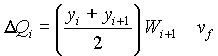
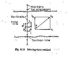
Fig. 4.15 Moving-boat method
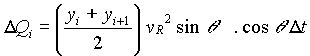 (4.11)
Thus by measuring the depths yi, velocity vR and q in a reach and the time taken to cross the reach D t, the discharge in the sub-area can be determined. The summation of the partial discharges D Qi over the whole width of the stream gives the stream discharge
Q = å D Qi (4.12)
In field applications a good stretch of the river with no shoals, islands, bars, etc. is selected. The cross-sectional line is defined by permanent land marks so that the boat can be aligned along this line. A motor boat with different sizes of outboard motors for use in different river stages is selected. A special current meter of the propeller-type, in which the velocity and inclination of the meter to the boat director 0 in the horizontal plane can be measured, is selected. The current meter is usually immersed at a depth of 0.5 m from the water surface to record surface velocities. To mark the various vertical sections and know the depths at these points, an echo-depth recorder is used.
In a typical run, the boat is started from the water edge and aligned to go across the cross-sectional line. When the boat is in sufficient depth of water, the instruments are lowered. The echo-depth recorder and current meter are commissioned. A button on the signal processor when pressed marks a distinctive mark line on the depth vs time chart of the echo-depth recorder. Further, it gives simultaneously a sharp audio signal to enable the measuring party to take simultaneous readings of the velocity vR and the inclination q . A large number of such measurements are taken during the traverse of the boat to the other bank of the river. The operation is repeated in the return journey of the boat. It is important that the boat is kept aligned along the cross-sectional line and this requires considerable skill on the part of the pilot. Typically, a river of about 2km stretch takes about 15 min for one crossing. A number of crossings are made to get the average value of the discharge. The surface velocities are converted to average velocities across the vertical by applying a coefficient [Eq. (4.5)]. The depths yi and time intervals D t are read from the echo-depth recorder chart. The discharge is calculated by Eqs. (4.11) and (4.12). In practical use additional coefficients may be needed to account for deviations from the ideal case and these depend upon the actual field conditions.
DILUTION TECHNIQUE OF STREAMFLOW MEASUREMENT
The dilution method of flow measurement, also known as the chemical method depends upon the continuity principle applied to a tracer which is allowed to mix completely with the flow. Consider a tracer which does not react with the fluid or boundary.
Let Co be the small initial concentration of the tracer in the streamflow. At section 1 a small quantity (volume V1) of high concentration C1 of this tracer is added (Fig. 4.16). Let section 2 be sufficiently far away on the downstream of section 1 so that the tracer mixes thoroughly with the fluid due to the turbulent mixing process while passing through the reach. The concentration profile taken at section 2 is schematically shown in Fig. 4.16. The concentration will have a base value of CO, increases from time t1 to a peak value and gradually reaches the base value of Co at time t2. The streamflow is assumed to be steady.
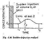
Fig. 4.16 Sudden-injection method
By continuity of the tracer material M1 = mass of tracer added at section 1 = V1 Cl
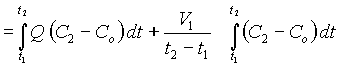
Neglecting the second term on the right-hand side as insignificantly small,
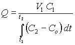 (4.13)
Thus the discharge Q in the stream can be estimated if for a known M1 the variation of C2 with time at section 2 and Co are determined. This method is known as sudden injection or gulp or integration method.
Another way of using the dilution principle is to inject the tracer of concentration C1 at a constant rate Qt at section 1. At section 2, the concentration gradually rises from the background value of Co at time t1 to a constant value C2 (Fig. 4.17). At the stready state, the continuity equation for the tracer is
![]()
i.e. 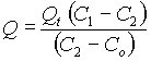 (4.14)
This technique in which Q is estimated by knowing C1, C2, Co and Q is known as constant rate injection method or plateau gauging.

Fig.4.17 Constant rate injection method
It is necessary to emphasise here that the dilution method of gauging is based on the assumption of steady flow. If the flow is unsteady and the flow rate changes appreciably during gauging, there will be a change in the storage volume in the reach and the steady-state continuity equation used to develop Eqs. (4.13) and (4.14) is not valid. Systematic errors can be expected in such cases.
Tracers
The tracer used should have ideally the following properties:
• It should not be absorbed by the sediment, channel boundary and vegetation. It
should not chemically react with any of the above surfaces and also should not be
lost by evaporation.
• It should be non-toxic.
• It should be capable of being detected in a distinctive manner in small
concentrations.
• It should not be very expensive.
The tracers used are of three main types:
• Chemicals (common salt and sodium dischromate are typical);
• Fluorescent dyes (Rhodamine-WT and Sulpho-Rhodamine B Extra are typical);
• Radioactive materials (such as Bromine-82, Sodium-24 and Iodine-132).
Common salt can be detected with an error of ± 1% up to a concentration of 10 ppm. Sodium dichromate can be detected up to 0.2 ppm concentrations. Fluorescent dyes have the advantage that they can be detected at levels of tens of nanograms per litre (~1 in 1011) and hence require very small amounts of solution for injections. Radioactive traces are detectable up to accuracies of tens of picocuries per litre (~1 in 1014) and therefore permit large-scale dilutions. However, they involve the use of very sophisticated instruments and handling by trained personnel only. The availability of detection instrumentation, environmental effects- of the tracer and overall cost of the operation are chief factors that decide the tracer to be used.
Length of Reach
The length of the reach between the dosing section and sampling section should be adequate to have complete mixing of the tracer with the flow. This length depends upon the geometric dimensions of the channel cross-section, discharge and turbulence levels. An empirical formula suggested by Rimmar (1960) for estimation of mixing length for point injection of a tracer in a straight reach is
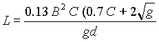 (4.15)
where L = mixing length (m), B = average width of the stream (m), d = average depth of the stream (m), C = Chezy coefficient of roughness which varies from 15 to 50 for smooth to rough bed conditions and g = acceleration due to gravity. The value of L varies from about 2 km for a mountain stream carrying a discharge of about 1.0 m³/s to about 100 km for river in a plain with a discharge of about 300 m³/s. The mixing length becomes very large for large rivers and is one of the major constraints of the dilution method. Artificial mixing of the tracer at the dosing station may prove beneficial for small streams in reducing the mixing length of the reach.
Use
The dilution method has the major advantage that the discharge is estimated directly in an absolute way. It is a particularly attractive method for small turbulent streams, such as those in mountainous areas. Where suitable, it can be used as an occasional method for checking the calibration, stage-discharge curves, etc. obtained by other methods.
ELECTROMAGNETIC METHOD
The electromagnetic method is based on the Faraday's principle that an emf is induced in the conductor (water in the present case) when it cuts a normal magnetic field. Large coils buried at the bottom of the channel carry a current I to produce a controlled vertical magnetic field, (Fig.4.18). Electrodes provided at the sides of the channel section measure the small voltage produced due to flow of water in the channel.
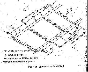
Fig. 4.18 Electromagnetic method
It has been found that the signal output E will be of the order of millivolts and is related to the discharge Q as
&#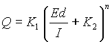 (4.16)
where d = depth of flow, I = current in the coil, and n, K1 and K2 are system constants.
The method involves sophisticated and expensive instrumentation and has been successfully tried in a number of installations. The fact that this kind of set-up gives the total discharge when once it has been calibrated, makes it specially suited for field situations where the cross-sectional properties can change with time due to weed growth, sedimentation, etc. Another specific application is in tidal channels where the flow undergoes rapid changes both in magnitude as well as in direction. Present-day commercially available electromagnetic flowmeters can measure the discharge to an accuracy of ±3%, the maximum channel width that can be accommodated being 100 m. The minimum detectable velocity is 0.005 m/s.
ULTRASONIC METHOD
This is essentially an area-velocity method with the average velocity being measured by using ultrasonic signals. The method was first reported by Swengel (1955); since then it has been perfected and complete systems are available commercially.
Consider a channel carrying a flow with two transducers A and B fixed at the same level h above the bed and on either sides of the channel (Fig. 4.19). These transducers can receive as well as send ultrasonic signals. Let A send an ultrasonic signal to be received at B after an elapse time t1.
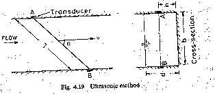
Fig. 4.19 Ultrasonic method
Similarly, let B send a signal to be received at A after an elapse time t2.
If C = velocity of sound in water,
![]() (4.17)
(4.17)
where L = length of path from A to B and vp = component of the flow velocity in the sound path = v cos q . Similarly, from Fig.4.19 it is easy to see that
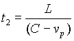 (4.18)
Thus 
Or 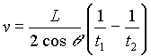 (4.19)
Thus for a given L and q , by knowing t1 and t2, the average velocity along the path AB, i.e. v can be determined. It may be noted that v is the average velocity at a height h above the bed and is not the average velocity V for the whole cross-section. However, for a given channel cross-section v can be related to V and by calibration a relation between v/V and h can be obtained. For a given set-up, as the area of cross-section is fixed, the discharge is obtained as a product of area and mean velocity V. Estimation of discharge by using one signal path as above is called single-path gauging. Alternatively, for a given depth of flow, multiple single paths can be used to obtain v for different h values. Mean velocity of flow through the cross-section is obtained by averaging these v values. This technique is known as multi-path gauging.
Ultrasonic flowmeters using the above principal have frequencies of the order of 500 kHz. Sophisticated electronics are needed to transmit, detect and evaluate the mean velocity of flow along the path. In a given installation a calibration (usually performed by the current-meter method) is needed to determine the system constants. Currently available commercial systems have been installed successfully at many places and accuracies of about 2% for the single-path method and 1% for the multipath method are reported. The systems are currently available for rivers up to 500 m width.
The specific advantages of the ultrasonic system of river gauging are:
• It is rapid and gives high accuracy;
• It is suitable for automatic recording of data;
• It can handle rapid changes in the magnitude and direction of flow as in tidal
rivers;
• The cost of installation is independent of the size of rivers.
The accuracy of this method is limited by the factors that affect the signal velocity and averaging of flow velocity, such as
• Unstable cross-section í fluctuating weed growth,
• High loads of suspended solids, í air entertainment and
• Salinity and temperature changes.
INDIRECT METHODS
Under this category are included those methods which make use of relationship between the flow discharge and the depths at specified locations. The field measurement is restricted to the measurement of t depths only. Two broad classifications of these indirect methods are:
• Flow measuring structures, and
• Slope area methods.
Flow-Measuring Structures
Use of structures like notches, weirs flumes and sluice gates for flow measurement in hydraulic laboratories is well known. These conventional structures are used in field conditions also but their use is limited by the ranges of head, debris or sediment load of the stream and the back-water effects produced by the installations. To overcome many of these limitations a wide variety of flow measuring structures with specific advantages are in use.
The basic principle governing the use of a weir, flume or similar flow measuring structure is that these structures produce a unique control section in the flow. At these structures, the discharge Q is a function of the water-surface elevation measured at a specified upstream location,
Q =f (H) (4.20)
where H = water surface elevation measured from a specified datum.
Thus, for example, for weirs, Eq. (4.20) takes the form
&#Q = K Hn (4.21)
where H = head over the weir and K, n = system constants. Equation (4.20) is applicable so long as the downstream water level is below a curtain limiting water level known as the modular limit. Such flows which are independent of the downstream water level are known as free flows. If the tailwater conditions do affect the flow, then the flow is known as drowned or submerged flow. Discharges under drowned condition are obtained by applying a reduction factor to the free flow discharges. For example, the sumberged flow over a weir (Fig. 4.20) is estimated by the Villemonte formula,
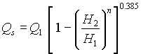 (4.22)
Where, Qs = submerged discharge, Q1 = free flow discharge under head H1, H1 = upstream water surface elevation measured above the weir crest, H2 = downstream water surface elevation measured above the weir crest, n exponent of head in the free flow head discharge relationship [ Eq. (4.21)]. For a rectangular weir n = 1.5.
The various flow measuring structures can be broadly considered under three categories:
Thin-plate structures are usually made from a vertically set metal plate. The V-notch, rectangular full width and contracted notches are typical examples under this category.
Long-base weirs, also known as broad-crested weirs are made of concrete or masonry and are used for large discharge values.
Flumes are made of concrete, masonry or metal sheets depending on their use and location. They depend primarily on the width constriction to produce a control section.
Fig. 4.20 Flow over a weir: (a) Free flow (b) Submerged flow
Slope-Area Method
The resistance equation for uniform flow in an open channel, e.g. Manning’s formula can be used to relate the depths at either ends of a reach to the discharge. Figure 4.21 shows the longitudinal section of the flow in a between two sections, 1 and 2. Knowing the water-surface elevations at the two sections, it is required to estimate the discharge.
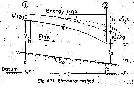
Fig. 4.21 Slope-area method
STAGE-DISCHARGE RELATIONSHIP
As indicated earlier the measurement of discharge by the direct method involves a two step procedure; the development of the stage-discharge relationship which forms the first step is of utmost importance. Once the stage-discharge (G-Q) relationship is established, the subsequent procedure consists of measuring the stage (G) and read the discharge (Q) from the (G-Q) relationship. This second part is a routine operation. Thus the aim of all current-meter and other direct-discharge measurements is to prepare a stage discharge relationship for the given channel gauging section. The stage-discharge relationship is also known as the rating curve.
The measured value of discharges when plotted against the corresponding stage give a relationship that represents the integrated effect of a wide range of channel and flow parameters. The combined effect of these parameters is termed control. If the (G-Q) relationship for a gauging section is constant and does not change with time, the control is said to be Permanent. If it changes with time, it is called shifting control.
Permanent Control
A majority of streams and rivers, especially nonalluvial rivers exhibit permanent control. For such a case, the relationship between the stage and the discharge is a single-valued relation, which is expressed as
Q = Cr (G - a)b (4.26)
in which Q = stream discharge, G = gauge height (stage), a = a constant which represent the gauge reading corresponding to zero discharge, Cr and b are rating curve constants. This relationship can be expressed graphically by plotting the observed stage against the corresponding discharge values in an arithmetic or logarithmic plot [Fig. 4.22 (a) and (b)] . Logarithmic plotting is advantageous as Eq. (4.26) plots as a straight line in logarithmic coordinates. In Fig. 4.22(b) the straight line is drawn to best represent the data plotted as Q vs (G-a). Coefficients Cr and b need not be the same for the full range of stages.
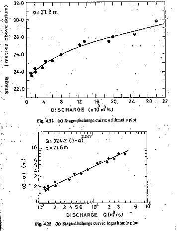
Fig. 4.22 (a) Stage-discharge curve: arithmetic plot
Fig. 4.22 (b) Stage-discharge curve: logarithmic plot
The best values of Cr and b in Eq. (4.26) for a given range of stage are obtained by the least-square-error method. Thus by taking logarithms,
log Q = b log (G - a) + log Cr (4.27)
or Y = b X + b (4.27a)
in which Y = log Q, X = log (G - a) and b = log Cr.
For the best-fit straight line of N observations of X and Y,
 (4.28)
and 
In the above it should be noted that a is an unknown and its determination poses some difficulties. The following alternative methods are available for its determination:
• Plot Q vs G on an arithmetic graph paper and draw a best-fit curve.
By extrapolating the curve by eye judgement find a as the value of G corresponding to Q = 0. Using this value of a, plot log Q vs log (G-a) and verify whether the data plots as a straight line. If not, select another value in the neighbourhood of previously assumed value and by trial and error find an acceptable value of a which gives a straight line plot of log Q vs log (G-a).
A graphical method due to Running' is as follows: The Q vs G data are plotted to an arithmetic scale and a smooth curve through the plotted points are drawn. Three points A, B and C on the curve are selected such that their discharges are in geometric progression, (Fig. 4.23) i.e.
At A and B vertical lines are drawn and then horizontal lines are drawn at B and C to get D and E as intersection points with the verticals. Two straight lines ED and BA are drawn to intersect at F.

Fig. 4.23 Running's method for estimation of the constant
The ordinate at F is the required value of a, the gauge height corresponding to zero discharge. This method assumes the lower part of the stage-discharge curve to be a parabola.
Plot Q vs G to an arithmetic scale and draw a smooth good-fitting curve by eye-judgement. Select three discharges Q1, Q2 and Q3, such that Q1/Q2 = Q2/Q3 and note from the curve the corresponding values of gauge readings G1, G2 and G3. From Eq. (4.27)
![]()
i.e.  (4.29)
A number of optimization procedures that are based on the use of computers are available to estimate the best value of a. A trial-and-error search for a which gives the best value of the correlation coefficient is one of them.
Shifting Control
The control that exists at a gauging section giving rise to a unique stage discharge relationship can change due to:
• Changing characteristics caused by weed growth, dredging or channel
encroachment, aggradation or degradation phenomenon in an alluvial channel,
• Variable backwater effects affecting the gauging section and
• Unsteady flow effects of a rapidly changing stage.
Backwater Effect
If the shifting control is due to variable backwater curves, the same stage indicates different discharges depending upon the backwater effect. To remedy this situation another gauge, called the secondary gauge or auxiliary gauge is installed some distance downstream of the gauging section and readings of both gauges are taken. The difference between the main gauge and the secondary gauge gives the fall (F) of the water surface in the reach. Now, for a given main-stage reading, the discharge under variable backwater condition is a function of the fall F, i.e.
&#Q = f (G, F) (4.30)
Schematically, this functional relationship is shown in Fig. 4.24. Instead of having a three-parameter plot, the observed data is normalized with respect to a constant fall value. Let Fo be a normalizing value of the fall 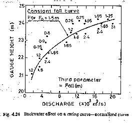
Fig. 4.24 Backwater effect on a rating curve-normalized curve
taken to be constant at all stages, F the actual fall at a given stage when the actual discharge is Q. These two fall values are related as
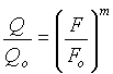 (4.31)
in which Qo = normalized discharge at the given stage when the fall is equal to Fo and m = an exponent with a value close to 0.5. From the observed data, a convenient value of Fo is selected. An approximate Qo vs G curve for a constant Fo called constant fall curve is drawn. For each observed data, Q/Qo and F/Fo values are calculated and plotted as Q/Qo vs F/Fo (Fig.4.25). This is called the adjustment curve. Both the constant fall curve and the adjustment curve are refined, by trial and error to get
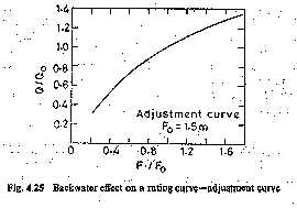
Fig. 4.25 Backwater effect on a rating curve-adjustment curve
the best-fit curves. When finalized, these two curves provide the stage-discharge information for gauging purposes. For example, if the observed stage is G1 and fall F1, first by using the adjustment curve the value of Q1/Qo is read for a known value of F1/Fo. Using the constant fall-rating curve, Qo is read for the given stage G1 and the actual discharge calculated as (Q1/Qo) x Qo.
Unsteady-Flow Effect
When a flood wave passes a gauging station in the advancing portion of the wave the approach velocities are larger than in the steady flow at corresponding stages. Thus for the same stage, more discharge than in a steady uniform flow occurs. In the retreating phase of the flood wave the converse situation occurs with reduced approach velocities giving lower discharges than in an equivalent steady flow case. Thus the stage-discharge relationship for an unsteady flow will not be a single-valued relationship as in steady flow but it will be a looped curve as in Fig. 4.26. It may be noted that at the same stage, more discharge passes through the river during rising stages than in falling ones. Since the conditions for each flood may be different, different floods may give different loops.
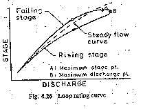
Fig. 4.26 Loop rating curve
If Qn is the normal discharge at a given stage under steady uniform flow and Qm is the measured (actual) unsteady flow the two are related as
 (4.32)
where So = channel slope = water surface slope at uniform flow, dh/dt = rate of change of stage and Vw = velocity of the flood wave. For natural channels, Vw is usually assumed equal to 1.4 V, where V = average velocity for a given stage estimated by applying Manning's formula and the energy slope Sf. Also, the energy slope is used in place of So in the denominator of Eq. (4.32). If enough field data about the flood magnitude and dh/dt are available, the term (1/Vw So) can be calculated and plotted against the stage for use in Eq. (4.32). For estimating the actual discharge at an observed stage, QM/Qn is calculated by using the observed data of dh/dt. Here Qn is the discharge corresponding to the observed stage relationship for steady flow in the channel reach.
EXTRAPOLATION OF RATING CURVE
Most hydrological designs consider extreme flood flows. As an example, in the design of hydraulic structures, such as barrages, dams and bridges one need maximum flood discharges as well as maximum flood levels. While the design flood discharge magnitude can be estimated from other considerations, the stage-discharge relationship at the project site will have to be used to predict the stage corresponding to design-flood discharges. Rarely will the available stage-discharge data include the design-flood range and hence the need for extrapolation of the rating curve.
Before attempting extrapolation, it is necessary to examine the site and collect relevant data on changes in the river cross-section due to flood plains, roughness and backwater effects. The reliability of the extrapolated value depends on the stability of the gauging section control. A stable control at all stages leads, to reliable results. Extrapolation of the rating curve in an alluvial river subjected to aggradations and degradation is un-reliable and the results should always be confirmed by alternate methods, There are many techniques of extending the rating curve and two well-known methods are described here.
Conveyance Method
The conveyance of a channel in nonuniform flow is defined by the relation
Q = K Ö St #9; #9; #9; (4.33)
where Q = discharge in the channel, St = slope of the energy line and K = conveyance. If Manning's formula is used,
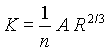 (4.34)
where n = Manning's roughness, A = area of cross-section and, R hydraulic radius. Since A and R are functions of the stage, the values of K for various values of stage are calculated by using Eq. (4.34) and plotted against the stage. The range of the stage should include values beyond the level up to which extrapolation is, desired. Then a smooth curve is fitted to the plotted points [Fig. 4.27(a)). Using the available discharge and stage data, values of St are calculated by using Eq. (4.33) as St = Q²/K² and are plotted against the stage. A smooth curve is fitted through the plotted points [Fig. 4.27(b)]. This curve is then extrapolated keeping in mind that Sf approaches a constant value at high stages.

Fig.4.27 Conveyance method rating curve extension: (a) K vs stage (b) Sf vs stage
Logarithmic-plot Method
In this technique the stage-discharge relationship by Eq.(4.26) is made use of. The stage is plotted against the discharge on a log-log paper. A best-fit linear relationship is obtained for data points lying in the high-stage range and the line is extended to cover the range of extrapolation. Alternatively, coefficients of Eq. (4.26) are obtained by the least-square-error method by regressing X on Y in Eq. (4.27a). For this Eq. (4.27a) is written as
X = a Y + C (4.35)
where X = log (G-a) and Y = log Q. The coefficients a and C are obtained as,
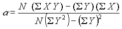 (4.35a)
and 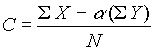 (4.35b)
The relationship governing the stage and discharge is now
(G - a) = Cl Qa (4.36)
where Cl= antilog C.
By the use of Eq. (4.36) the value of the stage corresponding to a design flood discharge is estimated.
RUNOFF
Runoff means the draining or flowing off of precipitation from a catchment area through a surface channel. It thus represents the output from the catchment in a given unit of time.
Consider a catchment area receiving precipitation. For a given precipitation, the evapotranspiration, initial loss, infiltration and detention-storage requirements will have to be first satisfied before the commencement of runoff. When these are satisfied, the excess precipitation moves over the lend surfaces to reach smaller channels. This portion of the runoff is called overland flow and involves building up of a storage over the surface and daining off of the same. Usually the lengths and depths of overland flow are small and the flow is in the larninar regime. Flows from several small channels join bigger channels and flows from these in turn combine to form a larger stream, and so on, till the flow reaches the catchment outlet. The flow in this mode where it travels all the time over the surface as over landflow and through the channels as open-channel flow and reaches the catchment outlet is called surface runoff.
A part of the precipitation that infilters moves laterally through upper crusts of the soil and returns to the surface at some location away from the point of entry into the soil. This component of runoff is known variously as interflow, through flow, storm seepage, subsurface, storm flow or quick return flow (Fig. 5.1). The amount of interflow depends on the biological conditions of the catchment. A fairly pervious soil overlying a hard impermeable surface is conducive to large interflows. Depending upon time delay between the infiltration and the outflow, the interflow is sometimes classified into prompt interflow, i.e. the interflow with the least time lag and delayed interflow.
Another route for the infiltered water is to undergo deep percolation and
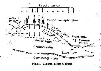
Fig. 5.1 Different routes of runoff
reach the groundwater storage in the soil. The groundwater follows a complicated and long path of travel, and ultimately reaches the surface. The time lag, i.e. the difference in time between the entry into the soil and outflows from it is very large, being of the order of months and years. This part of runoff is called groundwater runoff or groundwater. Ground water flow provides the dry-weather flow in perennial streams.
Based on the time delay between the precipitation and the runoff, the runoff is classified into two categories; as direct runoff and Base flow
Direct Runoff
It is that part of runoff which enters the stream immediately after the precipitation. It includes surface runoff, prompt interflow and precipitation the channel surface. In the case of snow-melt, the resulting flow entering the stream is also a direct runoff. Sometimes terms such as direct runoff and storm runoff are used to designate direct runoff.
Base Flow
The delayed flow that reaches a stream essentially as groundwater flow is called base flow. Many times delayed interflow is also included under this category.
Runoff, representing the response of a catchment to precipitation reflects the integrated effects of a wide range of catchment, climate and precipitation characteristics. True runoff is therefore stream flow in the natural condition, i.e. without human intervention. Such a stream flow unaffected by works of man, such as structures for storage and diversion on a stream is called virgin flow. When there exist storage or diversion works on a stream, the flow in the downstream channel is affected by structures and hence does not represent the true runoff unless corrected for storage effects and the diversion of flow and return flow.
HYDROGRAPH
A plot of the discharge in a stream plotted against time chronologically is called a Hydrograph. Depending upon the unit of time involved, we have:
Annual hydrographs showing the variation of daily or weekly or 10 daily mean flows over a year;
Monthly hydrogaphs showing the variation of daily mean flows over a month;
Seasonal hydrograps depicting the variation of the discharge in a particular season such, as the monsoon season or dry season; and
í Flood bydrographs or hydrographs due to a storm representing stream flow due to a storm over a catchment.
Each of these types have particular applications. Annual and seasonal hydrographs are of use in
• Calculating the surface water potential of stream,
• Reservoir studies and
• Drought studies.
Flood hydrographs are essential in analysing stream characteristics associated with floods.
Water Year
In annual runoff studies it is advantageous to consider a water year beginning from the time when the precipitation exceeds the average evapotranspiration losses. In India, June Ist is the beginning of a water year which ends on May 31st of the following calendar year. In a water year a complete cycle of climatic changes is expected and hence the water budget will have the least amount of carry over.
RUNOFF CHARACTERISTICS OF STREAMS
A study of the annual hydrographs of streams enables one to classify stream into three classes as perennial, intermittent and ephemeral. A perennial stream is one which always carries some flow (Fig. 5.2). There is considerable amount of groundwater flow throughout the year.
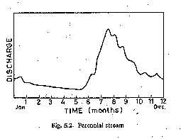
Fig. 5.2 Perennial stream
Even during dry seasons the water table will be above the bed of the stream.
An intermittent stream has limited contribution from the groundwater. During the wet season the water table is above the stream bed and there is a contribution of the base flow to the stream flow. However, during dry seasons the water table drops to a level lower than that of the stream bed and the stream dries up. Excepting for an occasional storm which can produce a short-duration flow, the stream remains dry for the most part of the dry months (Fig. 5.3).
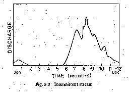
Fig. 5.3 Intermittent stream
An ephemeral stream is one, which does not have any base-flow contribution. The annual hydrograph of such a river show series of short-duration spikes marking flash flows in response to storms (Fig. 5.4). The stream becomes dry soon after the end of the storm flow. Typically an ephemeral stream does not have any well-defined channel. Most rivers in and zones are of the ephemeral kind,
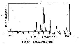
Fig. 5.4 Ephemeral stream
The flow characteristics of a stream depend upon:
The ranifall characteristics, such as magnitude intensity, distribution time and space and its variability;
Catchment characteristics such as soil, vegetation, slope, geology, shape and drainage density; and
The interrelationship of these factors is extremely complex. However, the risk of oversimplification, the following salient points can be noted:
The seasonal variation of rainfall is clearly reflected in the High stream discharges occur during monsoon months and 1ow which is essentially due to base flow is maintained during the year.
The shape of the storm hydrograph and hence the peak flow is essentially controlled by the storm and physical characteristics the catchment. Evapotranspiration plays a minor role in this.
The annual runoff volume (yield) of a stream is mainly controlled the amount of rainfall and evapotranspiration. The geology of catchment is significant to the extent of deep percolation losses.
YIELD (ANNUAL RUNOFF VOLUME)
The total quantity of water that can be expected from a stream in a given period such as a year is called the yield of the river. It is usual for yield to be referred to the period of a year and then it represents the annual runnoff volume. In this book the term yield is used to mean annual runoff volume unless otherwise specified. The calculation of yield is of fundamental importance in all water-resources development studies. The various methods used for the estimation of yield can be listed below:
Correlation of stream flow and rainfall,
Empirical equations, and
Watershed simulations.
Rainfall-Runoff Correlation
The relationship between rainfall and the resulting runoff is quite complex and is influenced by a host of factors relating the catchment and climate. Further, there is the problem of paucity of data which forces one to adopt simple correlations for the adequate estimation of runoff. One of the most common methods is to correlate runoff, R with rainfall, P values. Plotting of R values against P and drawing a best-fit line can be adopted for very rough estimates. A better method is to fit a linear regression line between R and P and to accept the result if the correlation coefficient is nearer unity. The equation for straight-line regression between runoff R and rainfall P is
R = a P + b (5.1)
and the values of the coefficients a and b are given by
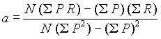 (5.2)
(5.2)
and 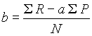 (5.3)
(5.3)
in which N = number of observation sets R and P. The coefficient of correlation r can be calculated as
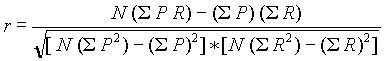 (5.4)
(5.4)
The value of r lies between 0 to + 1 as R can have only positive correlalion with P. A value of 0.6 < r < 1.0 indicates good correlation. Further it should be noted that R ³ 0.
For large catchments, it is found advantageous to have an exponential relationship as
R= b Pm (5.5)
where b and m are constants, instead of the linear relationship given by Eq. (5. 1). In that case Eq. (5.5) is reduced to a linear form by logarithmic transformation as
1n R = m 1n p + 1n b (5.6)
and the coefficients m and ln b determined by using the method indicated earlier,
Since rainfall records of longer duration than the runoff data are normally available for a catchment, the regression equation [(Eq. (5.1) or (5.5)] can be used to generate synthetic runoff data by using rainfall data. While this may be adequate for preliminary studies, for accurate results sophisticated methods are adopted for synthetic generation the runoff data. Many improvements of the above basic rainfall-runoff correlation by consider additional parameters such as soil moisture or antecedent rainfall have been attempted. Antecedent rainfall influences the initial soil moisture and hence the infiltration rate at the start of a storm. For calculation of the annual runoff from the annual rainfall a commonly used antecedent precipitation index, Pa is given by
Pa = a Pi + b Pi-1 + c Pi (5.7)
where Pi, Pi-1 and Pi-2 are the annual precipitation in the ith, (i-1)th (i-2)th year, i=current year, a, b and c are coefficients with their sum equal to unity. The coefficients are found by trial and error to produce best results.
There are many other types of antecedent precipitation indices in us achieve good correlations of rainfall and runoff. The use of coaxial chart with a defined antecedent precipitation index is given by Linsley et al.
Empirical Equations
The importance of estimating the water availability from, the available hydrologic data for purposes of planning water-resource projects was recognised by engineers even in the last century. With a keen sense of observation in their region of their activity many engineers of the past have developed empirical runoff estimation formulae. However, these formulae are applicable only to the region in which they were derived. These formulae are essentially rainfall-runoff relations with additional third or fourth parameters to account for climatic or catchement characteristics. Some of the important formulae used in various parts of India are given below.
Binnie's Percentages
Sir Alexander Bitinic measured the runoff from a small catchment near Nagpur (Area of 16 km2 ) during 1869 and 1872 and developed curves of cumulative runoff against cumulative rainfall. The two curves were found to be similar. From these he established percentages of runoff from rainfall. These percentages have been used in Madhya Pradesh and Vidarbha region of Maharashtra for the estimation of yield.
Barlow's Tables
Barlow, the first Chief Engineer of the Hydro-Electric Survey of India (1915) on the basis of his study in small catchments (area~ 130Km²)in Uttar Pradesh expressed runoff R as
R = Kb P (5.8)
Where Kb = runoff coefficient which depends upon the type of catchment and nature of monsoon rainfall.
Strange's Tables
Strange (1928) studied the then available data on rainfall and runoff in the border areas, of present-day Maharashtra and Karnataka and obtained the values of the runoff coefficient
&#Ks = R/P (5.9)
as a function of the catchment character. For purposes of calculating the yield from the total monsoon rainfall, the catchments were characterised as "good", "average" and "bad'. Values of Ks for these catchments are shown in Table 5.9. Strange also gave a table for calculating the daily runoff from daily rainfall. In this the runoff coefficient depends not only on the amount of rainfall but also on the state of the ground. Three categories of the original ground state as 'dry', 'damp' and 'wet' are used by him.
Iinglis and DeSouza Formula As a result of careful stream gauging in 53 sites in Western India, Inglis and DeSouza (1929) evolved two regional formulae between annual runoff R in cm and annual rainfall p in cm as follows:
• For Ghat regions of western India R = 0.85 P - 30.5 (5.10)
• For Deccan plateau
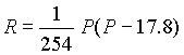 (5.11)
Khosla's Formula
Khosla (1960) analysed the rainfall, runoff and temperature data for various catchments in India and USA to arrive at an empirical relationship between runoff and rainfall. The time period is taken as a month. His relationship for Monthly runoff is
Rm = Pm - Lm (5.12)
and Lm = 0.48 Tm for Tm > 4.5°C
where Rm = Monthly runoff in cm and Rm 1 ³ 0
Pm = monthly rainfall in cm
Lm = monthly losses in cm
Tm = mean monthly temperature of the catchment in °C
For Tm £ 4.5°C, the loss Lm may provisionally be assumed as T°c 4.5 - 1 - 6.5, Lm (cm) 2.17 1.78 1.52 and Annual runoff = S Rm
Khosla's formula is indirectly based on the water-balance concept and the mean monthly catchment temperature is used to reflect the losses due to evapotranspiration. The formula has been tested on a number of catchments in India and is found to give fairly good results for the annual yield for use in preliminary studies. The formula can also be used to generate synthetic runoff data from historical rainfall and temperature data.
Watershed Simulation
The hydrologic water-budget equation for the determination of runoff a given period is written as
&#R = Rs + Go = P - Eet - D S (5.13)
in which Rs = surface runoff, P = precipitation, Eet = actual evapotranspiration, Go = net groundwater outflow and D S = change in the soilmoisture storage. The sum of Rs and Go is considered to be given by the total runoff R, i.e. streamflow.
Starting from an initial set of values, one can use Eq. (5.13) to calculate R by knowing values of P and functional dependence of Eet, D S and infiltration rates with catchment and climatic conditions. For accurate results, the functional dependence of various parameters governing the runoff in the catchment and values of P at short time intervals are needed. Calculations can then be done sequentially to obtain the runoff at any time. However, the calculation effort involved is enormous if attempted manually. With the availability of digital computers the use of water budgeting as above to determine the runoff has become feasible. This technique of predicting the runoff, which is the catchment response to a given rainfall input is called deterministic watershed simulation. In this the mathematical relationships describing the interdependence of various parameters in the system are first prepared and this is called the model. The model is then calibrated i.e. the numerical values of various coefficients determined, by simulating the known rainfall-runoff records. The accuracy of the model is further checked by reproducing the results of another string of rainfall data for which runoff values are known. This phase is known as validation or verification of the model. After this, the model is ready for use.
Crawford and Linsley (1959) pioneered this technique by proposing a watershed simulation model known as the Stanford Watershed Model (SWM). This underwent successive refinements and the Stanford Watershed Model-IV (SWM-IV) suitable for use on a wide variety of conditions was proposed in 1966. The flow chart of SWM-IV is shown in Figure 5.5. The main inputs are hourly precipitation and daily evapotranspiration in addition to physical description of the catchment. The model considers the soil in three zones with distinct properties to simulate evapotranspiration, infiltration, overland flow, channel flow, interflow and baseflow phases of the runoff phenomenon. For calibration about 5 years of data are needed. In the calibration phase, the initial guess value of parameters are adjusted on a trial-and-error basis until the simulated response matches the recorded values. Using an additional of rainfall-runoff of about 5 years duration, the model is verified for its ability to give proper response. A detailed description of the application of SWM to an Indian catchment is given in Ref. 3.
SWM-IV has been tested in a number of applications and it has been found to give satisfactory results for the yield and not so satisfactory results in predicting peak values. However, it requires considerable familiarity with the model to arrive at optimal values in the calibrating stage. An improved version called Hydrocomp Simulation Program (HSP) (1966) gives a package of three simulation modules to solve a variety of water-shed-simulation problems. Another model called the SSARR model (Streamflow Synthesis and Reservoir Regulation Model) developed by Rockwood (1968) for the Columbia river basin, USA has been successfully tested on large watersheds. The Kentucky Watershed model (KWM) (1 970) is a revised and updated version of SWM-IV. KWM is used with an optimization programme called OPSET which generates best-fit parameter estimates. The successful use of KWM to catchments up to 1200 km² size have been reported.
FLOW-DURATION CURVE
It is well-known that the streamflow varies over a water year. One of the popular methods of studying this streamflow variability is through flow a duration curves. A flow-duration curve of a stream is a plot of discharge against the per cent of time the flow was equalled or exceeded. This curve is also known as discharge-frequency curve.
The streamflow data is arranged in a descending order of discharges, using class intervals if the number of individual values is very large. The data used can be daily, weekly, ten daily or monthly values. If N number of data points are used in this listing, the plotting position of any discharge (or class value) Q is
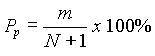 (5.14)
where m is the order number of the discharge (or class value), Pp = percentage probability of the flow magnitude being equalled or exceeded. The plot of the discharge Q against Pp is the flow-duration curve (Fig. 5.6). Arithmetic scale paper, or semi-log or log-log paper is used depending upon the range of data and use of the plot. The flow-duration curve represents the cumulative frequency distribution and can be considered to represent the streamflow variation of an average year. The ordinate Qp at any percentage probability Pp, represents the flow magnitude in an average year that can be expected to be equalled or exceeded Pp percent of time and is termed as Pp% dependable flow. In a perennial river Q100 = 100% dependable flow is a finite value. On the other hand in an intermittent or ephemeral river the streamflow is zero for a finite part of an year and as such Q100 is equal to zero.
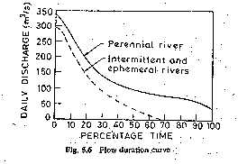
Fig. 5.6 Flow-duration curve
The following characteristics of the flow-duration curve are of interest:
The slope of a flow-duration curve depends upon the interval of selected. For example, a daily stream flow data gives a steeper curve than a curve based on Monthly data for the same stream. This is due to the smoothening' of small peaks in monthly data.
The presence of E.I. reservoir in a stream considerably modifies the virgin-flow-duration curve depending on the nature of flow regulation.
Figure 5.7 shows the typical reservoir regulation effect.
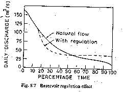
Fig. 5.7 Reservoir regulation effect
The virgin-flow-duration curve when plotted on a log probability paper plots as a straight line at least over the central region. From this property, various coefficients expressing the variability of the flow in a stream can be developed for the description and comparison of different streams.
The flow-duration curve plotted on a log-log paper (Fig. 5.8) is useful in comparing the flow characteristics of different streams. A steep slope of the curve indicates a stream with a highly variable discharge. On the other hand, a flat slope indicates a slow response of the catchment to the rainfall and also indicates small variability. At the lower end of the curve, a flat portion indicates considerable base flow. A fiat curve on the upper portion is typical of river basins having large flood plains and also of rivers baying large snowfall during a wet season.
Flow-duration curves find considerable use in water-resources planning and development activities. Some of the important uses are :
In evaluating various dependable flows in the planning or water-resources engineering projects;
In evaluating the characteristics of the hydropower potential of a river;
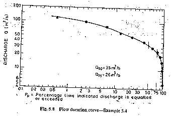
Fig. 5.8 Flow-duration curve
• In the design of drainage systems;
• In flood-control studies;
• In computing the sediment load and dissolved solids load of a stream; and
• In comparing the adjacent catchments with a view to extend the streamflow data.
FLOW-MASS CURVE
The flow-mass curve is a plot of the cumulative discharge volume against time Plotted in chronological order. The ordinate of the mass curve, V at any time t is thus
 (5.15)
where `to’ is the time at the beginning of the curve and Q is the discharge rate. Since the hydrograph is a plot of Q vs t, it is easy to see that the flow-mass-curve is an integral curve (summation curse) of the hydrograph. The flow-mass curve is also known as Rippl’s mass curve after Rippl (1882) who suggested its use first. Figure 5.9 shows a typical flow-mass curve. Note that the abscissa is chronological time in months in this figure. It can also be in days, weeks or months depending on the data being analysed. The ordinate is in units of volume in million m³. Other units employed for ordinate include m³/s. day (cumec day), ha.m and cm over a catchment area.
The slope of the mass curve at any point represents dV/dt = Q = rate of flow at that instant. If two points M and N are connected by a straight
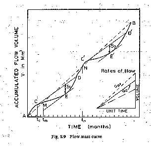
Fig. 5.9 Flow mass curve
line, the slope of the line represents the average rate of flow that can be maintained between the times tm and tn if a reservoir of adequate storage is available. Thus the slope of the line AB joining the first and the last points of a mass curve represents the average discharge over the whole period of plotted record.
HYDROGRAPHS
Consider a concentrated storm producing a fairly uniform rainfall of duration, Tr over a catchment. After the initial losses and infiltration losses are met, the rainfall excess reaches the stream through overland and channel flows. In the process of translation a certain amount of storage is built up in the overland and channel-flow phases. This storage gradually depletes after the cessation of the rainfall. Thus there is a time Jag between the occurrence of rainfall in the basin and the time when that water passes the gauging station at the basin outlet. The runoff measured at the stream gauging station will give a typical hydrograph as shown in Fig. 6.1. The duration of the rainfall is also marked in this figure to indicate the time lag in the rainfall and runoff. The hydrograph of this kind which results due to an isolated storm is typically single-peaked skew distribution of discharge and is known variously as storm hydrograph, flood hydrograph or simply hydrograph. It has three characteristic regions : (i) the rising limb AB, joining point A, the starting point of the rising curve and point B, the point of inflection, (ii) the crest segment BC between the two inflection with a peak P in between, (iii) the falling limb or depletion curve CD starting from the second point of inflection C. Other points of interest are tpk, the time to peak from the starting point A, the time from the centre of mass of rainfall to the centre of mass of hydrograph called lag time TL, the peak discharge Qp and the time base of the hydrograph TB.
The hydrograph is the response of a given catchment to a rainfall input.
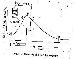
Fig.6.1 Elements of a flow hydrograph
It consists of flow in all the three phases of runoff, viz. surface runoff, interflow and base flow, and embodies in itself the integrated effects of a wide variety of atchnient and rainfall parameters having complex inter-actions. Thus two different storms in a given catchment Produce hydrhographs differing from each other. Similarly, identical storms in two catecments produce hydrographs that are different. The interactions of various storms and catchments are in general extremely complex. If one examines the record of a large number of flood hydrographs of a stream, it will be found that many of than will have kinks, multiple peaks, etc. resulting in shapes much different from the simple single-peaked hydrograph of Fig. 6.1. These complex hydrographs are the result of storm and catchment Peculiarities and their complex interactions. While it is theoretically possible to resolve a complex hydrograph into a set of simple hydro-graphs for purposes of hydrograph analysis, the requisite data of accept-able quality are seldom available. Hence, simple hydrographs resulting from isolated storms are preferred for hydrograph studies.
FACTORS AFFECTING FLOOD HYDROGRAPH
The factors that affect the shape of the hydrograph can be broadly grouped into climatic factors and physiographic factors. Each of these two groups contain a host of factors and the important on Table 6.1. Generally, the climatic factors control the rising limb and the recession limb is independent of storm characteristics, being determined by catchment characteristics only. Many of the factors listed in Table 6.1 are interdependent. Further, their effects are very varied and complicated. As such only important effects are listed below in qualitative terms only.
FACTORS AFFECTING FLOOD HYDROGRAPH
Physiographic Factors
• Basin characteristics : shape, size, slope, nature of the valley, elevation,
drainage density
• Infiltration characteristic : landuse and cover, soil type and geological conditions,
lakes, swamps and other storage
• Channel characteristics : crosssection, roughness and storage capacity.
Climatic Factors
• Storm characteristics: precipitation, intensity, duration, magnitude and movement
of Storm.
• Initial loss
• Evapotranspiration
Shape of the Basin
The shape of the basin influences the time taken for water from the remote parts of the catchment to arrive at the outlet. Thus the occurrence of the peak and hence the shape of the hydrograph are affected by the basin shape. Fan-shaped, i.e. nearly semi-circular shaped catchments give high peak and narrow hydrographs while elongated catchments give broad-and low-peaked hydrographs. Figure 6.2 shows schematically the hydrographs from
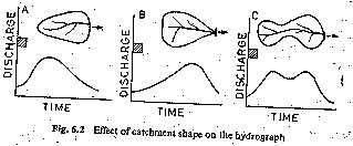
Fig. 6.2 Effect of catchment shape on the hydrograph
three catchments having identical infiltration characteristics due to identical rainfall over the catchment. In catchment A the hydrograph is skewed to the left, i.e. the peak occurs relatively quickly. In catchment B, the hydrograph is skewed to the right, the peak occurring with a relatively longer lag. Catchment C indicates the complex hydrography produced by a composite shape.
Size
Small basins behave different from the large ones in terms of the relative importance of various phases of the runoff phenomenon. In small catchments the overland flow phase is predominant over the channel flow. Hence the land use and intensity of rainfall have important role on the peak good. On large basins these effects are suppressed as the channel flow phase is more predominant. The peak discharge is found to vary as An where A is the catchment area and n is an exponent whose value is less than unity, being about 0.5. The time base of the hydrographs from larger basins will be larger than those of corresponding hydrographs from smaller basins. The duration of the surface runoff from the time of occurrence of the peak is proportional to Am, where m is an exponent less than unity and is of the order of magnitude of 0.2.
Slope
The slope of the main stream controls the velocity of now in the channel. As the recession limb of the hydrograph represents the depletion of storage, the stream channel slope will have a pronounced effect on this part of the hydrograph. Large stream slopes give rise to quicker depletion of storage and hence result in steeper recession limbs of hydrographs. This would obviously result in a smaller time base.
The basin slope is important in small catchments where the overland low is relatively more important. In such cases the steeper slope of the catchment results in larger peak discharges.
Drainage Density
The drainage density is defined as the ratio of the total channel length to the total drainage area. A large drainage density creates situation conducive for quick disposal of runoff down the channels. This fast response is reflected in a pronounced peaked discharge. In basins with smaller drainage densities, the overland flow is predominant and the resulting hydrograph is squat with a slowly rising limb (Fig. 6.3).
Land Use
Vegetation and forests increase the infiltration and storage capacities of the Soils. Further, they cause considerable retardance to the overland flow. Thus the vegetal cover reduces the peak flow. This effect is usually very Pronounced in small catchments of area less than 150 km². Further, the effect of the vegetal cover is prominent in small storms. In general, for two catchments of equal area, other factors being identical, the peak discharge is higher for a catchment that has a lower density of forest cover. Of the various factors that control the peak discharge, probably the only factor that can be manipulated is land use and thus it represents the only practical means of exercising long-term natural control over the flood hydrograph of a catchment.
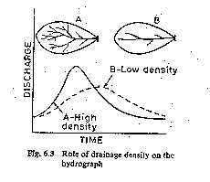
Fig. 6.3 Role of drainage density on the hydrograph
Climatic Factors
Among climatic factors the intensity, duration and direction of storm movement are the three important ones affecting the shape of a flood hydrograph. For a given duration, the peak and volume of the surface runoff are essentially proportional to the intensity of rainfall. This aspect is made use of in the unit hydrograph theory of estimating peak-flow hydrographs, as discussed in subsequent sections of this chapter. In very small catchments, the shape of the hydrograph can also be affected by the intensity.
The duration of a storm of given intensity also has a direct proportional effect on the volume of runoff. The effect of duration is reflected in the rising limb and peak flow. Ideally, if a rainfall of given intensity i lasts sufficiently long enough, a state of equilibrium discharge proportional to iA is reached.
If the storm moves from upstream of the catchment to the downstream end, there will be a quicker concentration of flow at the basin outlet. This results in a peaked hydrograph. Conversely, if the storm movement is up the catchment, the resulting hydrograph will have a lower peak and longer time base. This effect is further accentuated by the shape of the catchment, with long and narrow catchments having hydrographs most sensitive to the storm-movement direction.
COMPONENTS OF A HYDROGRAPH
As indicated earlier, the essential Components of a hydrograph are:
Rising limb,
Crest segment, and
Recession limb.
Rising Limb
The rising limb of a hydrograph, also known as concentration curve represents the increase in discharge due to the gradual building up of storage in channels and over the catchment surface. The initial losses and high infiltration losses during the early period of a storm cause the discharge to rise rather slowly in the initial periods. As the storm continues, more and more flow from distant parts reach the basin outlet. Simultaneously the infiltration losses also decrease with time. Thus under a uniform storm over the catchment, the runoff increases rapidly with time. As indicated earlier, the basin and storm characteristics control the shape of the rising limb of a hydrograph.
Crest Segment
The crest segment is one of the most important parts of a hydrograph as it contains the peak flow. The peak flow occurs when the runoff from various parts of the catchment simultaneously contribute the maximum amount of flow at the basin outlet. Generally for large catchments, the peak flow occurs after the cessation of rainfall, the time interval from the centre of mass of rainfall to the peak being essentially controlled by basin and storm characteristics. Multiple-peaked complex hydrographs in a basin can occur when two or more storms occur in close succession. Estimation of the peak flow and its occurrence, being very important in flood-flow studies are dealt in detail elsewhere in this book.
Recession Limb
The recession limb which extends from the point of inflection at the end of the crest segment to the commencement of the natural groundwater flow represents the withdrawal of water from the storage built up in the basin during the earlier phases of the hydrograph. The starting point of the recession limb, i.e. the point of inflection represents the condition of maximum storage. Since the depletion of storage takes place after the cessation of rainfall, the shape of this part of the hydrograph is independent of storm characteristics and depends entirely on the basin characteristics.
The storage of water in the basin exists as surface storage, which includes both surface detention and channel storage, interflow storage, and groundwater storage, i.e. base-flow storage. Barnes (1940) showed that the recession of a storage can be expressed as
![]() (6.1)
(6.1)
in which Qo and Qt are discharges at a time interval of t days with Qo being the initial discharge; Kr is a recession constant of value less than unity. Equation (6.1) can also be expressed in an alternative form of the exponential decay as
![]() (6.2)
(6.2)
![]() Where, a = - 1n Kr
Where, a = - 1n Kr
The recession constant Kr can be considered to be made up of three components to take care of the three types of storage as
Kr = Krs . Kri . Krb (6.3)
where Krs = recession constant for surface storage, Kri = recession constant for interflow and Krb = recession constant for base flow. Typically the values of these recession constants, when t is in days, are
Krs = 0.05 to 0.20
Kri = 0.50 to 0.85
Krb = 0.85 to 0.99
If the interflow is not significant Kri can be assumed to be unity. When Eq. (6.1) or (6.2) is plotted on a semilog paper with the discharge on the log-scale, it plots as a straight line and from this the value of Kr can be found.
EFFECTIVE RAINFALL
For purposes of correlating DRH with the rainfall which produced the flow, the hydrograph of the rainfall is also pruned by deducting the losses. Figure 6.6 shows the hyetograph of a storm. The initial loss and infiltration losses are subtracted from it. The resulting hyetograph is known as effective rainfall hyetograph (ERH). It is also known as hyetograph of rainfall excess or supra rainfall. Both DRH and ERH represent the same total quantity but in different units. Since ERH is usually in cm/h plotted against time, the area of ERH multiplied by the catchment area gives Fig. 6.6 the total volume of direct runoff, which is the same as the area of DRH. The initial loss and infiltration losses are estimated based on the available data of the catchment.
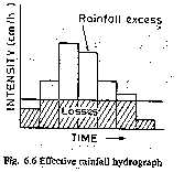
Fig.6.6 Effective rainfall hydrograph.
UNIT HYDROGRAPH
The problem of predicting the flood hydrograph resulting from a known storm in a catchment has received considerable attention. A large number of methods are proposed to solve this problem and of them probably the most popular and widely used method is the unit-hydrograph method. This method was first suggested by Sherman in 1932 and has undergone many, refinements since then.
A unit hydrograph is defined as the hydrograph of direct runoff resulting from one unit depth (1 cm) of rainfall excess occurring uniformly over the basin and at a uniform rate for a specified duration (Dh). The term unit here refers to a unit depth of rainfall excess which is usually taken as 1 cm. The duration, being a very important characteristic, is used as a prefix to a specific unit hydrograph. Thus one has a 6-h unit hydrograph, 12-h unit hydrograph, etc. and in general a D-h unit-hydrograph applicable to a given catchment. The definition of a unit hydrograph implies the following:
The unit hydrograph represents the lumped response of the catchment to a unit rainfall excess of D-h duration to produce a direct-runoff hydrograph. It relates only the direct runoff to the rainfall excess. Hence the volume of water contained in the unit hydrograph must be equal to the rainfall excess. As 1 cm depth of rainfall excess is considered the area of the unit hydrograph is equal to a volume given by 1 cm over the catchment.
The rainfall is considered to have an average intensity of excess rainfall (ER) of 1/D cm/h for the duration of the storm.
The distribution of the storm is considered to be uniform all over the catchment.
Fig.6.8 shows a typical 6-h unit hydrograph. Here the duration of the rainfall excess is 6 h.
Area under the unit hydrograph = 12.92 X 10⁶m³
Hence Catchment area of the basin = 12.92 km²
Two basic assumptions constitute the foundations for the unit hydrograph theory. These are the time invariance and the linear response.
Time Invariance
This first basic assumption is that the direct-runoff response to a given effective rainfall in a catchment is time-invariant. This implies that the DRH for a given ER in a catchment is always the same irrespective of when it occurs.
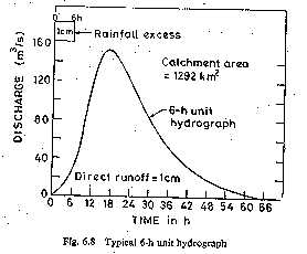
Fig. 6.8 Typical 6-h unit hydrograph
Linear Response
The direct-runoff response to the rainfall excess is assumed to be linear. This is the most important assumption of the unit-hydrograph theory. Linear response means that if an input x1(t) causes an output y1(t) and an input x2(t) causes an output y2(t), then an input x1(t)+x2(t) gives an output Yl(t)+Y2(t). Consequently, if X2(t) = rxl(t), then y2(t) = ry1(t). Thus if the rainfall excess in a duration D is r times the unit depth, the resulting DRH will have ordinates bearing ratio r to those of the corresponding D-h unit hydrograph. Since the area of the resulting DRH should increase by the ratio r, the base of the DRH will be the same as that of unit hydrograph.
The assumption of linear response in a unit hydrograph enables method of superposition to be used to derive DRHs. Accordingly, rainfall excesses of D-h duration each occur consecutively, their combined effect is obtained by superposing the respective DRHs with due cart taken to account for the Proper sequence of events. These aspects resulting from the assumption of linear response are made clearer following two illustrative examples.
DERIVATION OF UNIT HYDROGRAPHS
A number of isolated storm hydrographs caused by short spells of rainfall excess, each of approximately same duration [0.90 to 1.1 Dh] are selected from a study of the continuously gauged runoff of the stream. For each in these surface hydrographs, the base flow is separated by adopting one the methods indicated in Sec.6.4. The area under each DRH is evaluated and the volume of the direct runoff obtained is divided by the catchment area to obtain the depth of ER. The ordinates of the various DRHs are divided by the respective ER values to obtain the ordinates of the unit hydroraph.
Flood hydrographs used in the analysis should be selected to meet the following desirable features with respect to the storms responsible for them:
í The storms should be isolated storms occurring individually.
í The rainfall should be fairly uniform during the duration and should cover the entire catchment area.
í The duration of the rainfall should be 1/5 to 1/3 of the basin lag.
í The rainfall excess of the selected storm should be high. A range ER values of 1.0 to 4.0 cm is sometimes preferred.
A number of unit hydrographs of a given duration are derived by the above method and then plotted on a common pair of axes as shown in Fig.6.1 1. Because of rainfall variations both in space and time due to some departures from the assumptions of the unit-hydrograph theory, the various unit hydrographs thus developed will not be identical is common practice to adopt a mean of such curves as the unit graph of a given duration for the catchment. While deriving the mean curve, the average of peak flows and time to peaks are first calculated. Then a mean curve of best fit, judged by eye, is drawn through the averaged peak to close on an averaged base length. The volume of DRH is calculated and any departure from unity is corrected by adjusting the value of the peak. The averaged ERH of unit depth is customarily drawn in the plot of the unit hydrograph to indicate the type and duration of rainfall causing the unit hydrograph.
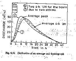
Fig. 6.11 Derivation of an average unit hydrograph
By definition the rainfall excess is assumed to occur uniformly over the catchment during duration D of a unit hydrograph. An ideal duration for a unit hydrograph is one wherein small fluctuations in the intensity of rainfall within this duration do not have any significant effects on the run-off. The catchment has a damping effect on the fluctuations of the rainfall intensity in the runoff-producing process and this damping is a function of the catchment area. This indicates that larger durations are admissible for larger catchments. By experience it is found that the duration of the unit hydrograph should not exceed 1/5 to 1/3 basin lag. For catchments of sizes larger than 250 km² the duration of 6h is generally satisfactory.
Unit Hydrograph from a Complex Storm
When suitable simple isolated storms are not available, data from complex storms of long duration will have to be used in unit-hydrograph derivation. The problem is to decompose a measured composite flood hydrograph into its component DRHs and base flow. A common unit hydrograph of appropriate duration is assumed to exist. This problem is thus the inverse of the derivation of flood hydrograph through use of Eq. (6.5). Consider a rainfall excess made up of three consecutive durations of D-h and ER values of R1, R2 and R3. Figure 6.13 shows the ERH. By base flow separation of the resulting composite flood hydrograph a composite DRH is obtained (Fig.6.13). Let the ordinates of the composite DRH be drawn at a time interval of D h. At various time intervals 1D, 2D, 3D, ...from the start of the ERH, let the ordinates of the unit hydrograph be u1, u2, u3, ... and the ordinates of the composite DRH be Ql, Q2, Q3 ...
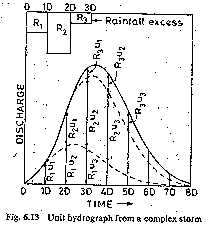
Fig. 6.13 Unit hydrograph from a complex storm
Then
Q1 = R1u1
Q2 = R1u2 + R2 ul
Q3 = R1u 3 + R2 u2 + R3 ul (6.6)
Q4 = R1u4 + R2 u3 + R3 u2
Q5 = R1u5 + R2 u4 + R3 u3
.................……………….
so on.
From the Eq.(6.6) the values of ul, u2, u3, ... can be determined. However, this method suffers from the disadvantage that the errors propagate and increase as the calculations proceed. In the presence of errors the recession limb of the derived D-h unit hydrograph can contain oscillations and even negative values. Matrix methods with optimisation schemes are available for solving Eq. (6.6) in a digital computer.
UNIT HYDROGRAPHS OF DIFFERENT DURATIONS
Ideally, unit hydrographs are derived from simple isolated storms and if the duration of the various storms do not differ very much, say within a band width of ± 20% D, they would all be grouped under one average duration of D h. If in practical applications unit hydrographs of different duration are needed they are best derived from field data. Lack of adequate data normally precludes development of unit hydrographs covering a wide range of durations for a given catchment. Under such conditions a D-h unit hydrograph is used to develop unit hydrographs of differing durations, nD. Two methods are available for this purpose i.e. Method of superposition, and S-curve.
Method of Superposition
If a D-h unit hydrograph is available, and it is desired to develop a unit hydrograph of nD h, where n is an integer, it is easily accomplished by superposing n unit hydrographs with each graph separated from the previous one by D h. Figure 6.14 shows three 4-h
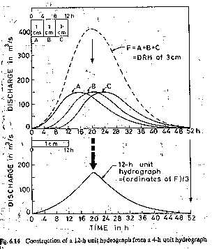
Fig.6.14 Construction of a 12-h unit hydrograph from a 4-h unit hydrograph
Unit hydrographs A, B and C, Curve B begins 4-h after B. Thus the combination of these three curves is a DRH of 3cm due to an ER of 12h duration. If the ordinates of this DRH art now divided by 3, one obtains a 12-h unit hydrograph. The calculations easy if performed in a tabular form (Table 6.6).
The S-Curve
If it is desired to develop a unit hydrograph of duration mD, where m is a fraction, the method of superposition cannot be used. A different technique known as the S-curve method is adopted in such cases, and this method is applicable for rational values of m.
The S-curve, also known as S-hydrograph is a hydrograph produced by a continuous effective rainfall at a constant rate for an infinite period. It is a curve obtained by summation of an infinite series of D-h unit hydrographs spaced D-h apart. Figure 6.15 shows such a series of D-h hydrograph arranged with their starting points D-h apart. At any given time the ordinates of the various curves occurring at that time coordinate are summed up to obtain ordinates of the S-curve. A smooth curve through these ordinates result in an S-shaped curve called S-curve.
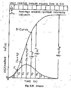
Fig. 6.15 S-Curve
This S-Curve is due to a D-h unit hydrograph. It has an initial steep portion and reaches a maximum equilibrium discharge at a time equal to the tine base of the first unit hydrograph. The average intensity of ER producing the S-curve is 1/D cm/h and the equilibrium discharge,
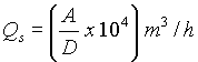
where A = area of the catchment in km² and D = duration in hours of ER of the unit hydrograph used in deriving the S-curve. Alternatively
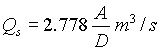 (6.7)
(6.7)
where A is in km² and D is in h. The quantity Qs represents the maximum rate at which an ER intensity of 1/D cm/h can drain out of a catchment of area A. In actual construction of an S-curve, it is found that curve oscillates in the top portion at around the equilibrium value due t magnification and accumulation of small errors in the hydrograph. When it occurs, an average smooth curve is drawn such that it reaches a value Qs at the time base of the unit hydrograph.
Consider two D-h S-curves A and B displaced by Th (Fig.6.16) If the ordinates of B are subtracted from that of A, the resulting curve is a DRH produced by a rainfall excess of duration T h and magnitude (1/D x T) cm. Hence if the ordinate differences of A and B, i.e. (SA – SB) are divided by T/D, the resulting ordinates denote a hydrograph due to an ER of 1 cm and of duration T h, i.e. a T-h unit hydrograph. The derivation of a T-h unit hydrograph as above can be achieved either by graphical mean arithmetic computations in a tabular form.
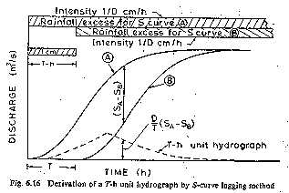
Fig. 6.16 Derivation of a T-h unit hydrograph by S-curve lagging method
USE AND LIMITATIONS OF UNIT HYDROGRAPH
As the unit hydrographs establish a relationship between the ERH and DRH for a catchment, they are of immense value in the study of the hydrology of a catchment. They are of great use in
Unit hydrographs assume uniform distribution of rainfall over the catchment. Also, the intensity is assumed constant for the duration of the unfair excess. In practice, these two conditions are never strictly satisfied. Nonuniform areal distribution and variation in intensity within a storm are very common. Under such conditions unit hydrographs can still be used if the areal distribution is consistent between different storms. However, the size of the catchment imposes an upper limit on the applicability of the unit hydrograph. This is because in very large basins the centre of the storm can vary from storm to storm and each can give different DRHs under otherwise identical situations. It is generally felt that about 500 km² is the upper limit for unit-hydrograph use. Flood hydrographs in very large basins can be studied by dividing then into a number of smaller subbasins and developing DRHs by the unit-hydrograph method. These DRHs can then be routed through their respective channels to obtain the composite DRH at the basin outlet.
There is a lower limit also for the application of unit hydrographs. This limit is usually taken as about 200 ha. At this level of area, a number of factors affect the rainfall-runoff relationship and the unit hydrograph not accurate enough for the prediction of DRH.
Other limitations to the use of unit hydrographs are:
Precipitation must be from rainfall only. Snow-melt runoff cannot be satisfactorily represented by unit hydrograph.
The catchment should not have unusually large storages in terms of tanks, ponds, large flood-bank storages, etc. which affect the line relationship between storage and discharge.
In the use of unit hydrographs very accurate reproduction of results should not be expected. Variations in the hydrograph base of as much as ± 200% and in the peak discharge by ± 10% are normally considered acceptable.
DURATION OF THE UNIT HYDROGRAPH
The choice of the duration of the unit hydrograph depends on the records. If recording raingauge data, are available any convenient depending on the size of the basin can be used. The choice is not only daily rainfall records are available. A rough guide for the choice of duration D is that it should not exceed the least of
(i)Time (ii) Basin lag and (iii) Time of concentration.
A value of D equal to about 1/4 of the basin lag is about the best choice. Generally, for with areas more than 1200 km² a duration D = 12 hrs is preferred.
DISTRIBUTION GRAPH
The distribution graph introduced by Bernard (1935) is a variation of unit hydrograph. It is basically a D-h unit hydrograph with ordinates showing the percentage of the surface runoff occurring in successive periods of equal time intervals of Dh. The duration of the rainfall excess (Dh) is taken as the unit interval and distribution-graph ordinates indicated at successive such unit intervals. Figure 6.17 shows a typical distribution graph. Note the ordinates plotted at 4-h intervals and the area under the distribution graph adds up to 100%. The use of the distribution graph to generate a DRH for a known ERH is exactly the same that of a unit hydrograph (Example 6.11). Distribution graphs are useful in comparing the runoff characteristics of different catchments.
SYNTHETIC UNIT HYDROGRAPH
To develop unit hydrographs to a catchment, detailed information about the rainfall and the resulting flood hydrograph are needed. However, such information would be available only at a few locations and in a majority of catchments, especially those which are at remote locations, the data would normally be very scanty. In order to construct unit hydrographs for such areas, empirical equations of regional validity which relate the salient hydrograph characteristics to the basin characteristics are available. Unit hydrographs derived from such relationships are known as synthetic-unit hydrographs. A number of methods for developing synthetic-unit hydrographs are reported in literature. It should, however, be re-numbered that these methods being based on empirical correlation’s are applicable only to the specific regions in which they were developed and could not be considered as general relationships for use in all regions.
INSTANTANEOUS UNIT HYDROGRAPH (IUH)
The unit-hydrograph concept discussed in the preceding sections considered a D-h unit hydrograph. For a given catchment a number of unit hydrographs of different durations are possible. The shape of these different unit hydrographs depend upon the value of D. Figure 6.20 shows a typical variation of the shape of unit hydrographs for different values of D. As D is reduced, the intensity of rainfall excess being equal to 1/D increases and the unit hydrograph becomes more skewed. A finite unit hydrograph is indicated as the duration DÕ 0. The limiting case of a unit hydrograph of zero duration is known as instantaneous unit hydrograph (IUH). Thus IUH is a fictitious, conceptual unit hydrograph which
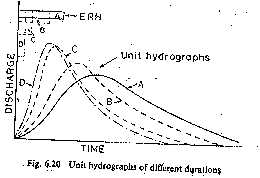
Fig. 6.20 Unit hydrographs of different duration
Represents the surface runoff from the catchment due to an instantaneous precipitation of the rainfall excess volume of 1 cm. IUH is designed u (t) or sometimes as u (0, t). It is a single-peaked hydrograph with a finite base width and its important properties can be listed as below:
1. 0 £ u (t) £ a positive value, for t > 0;
2. u (t) = 0 for t £ 0;
3. u (t) ® 0 as t ® a ;
4.  = unit depth over the catchment; and
_. time to the peak < time to the centroid of the curve.
Consider an effective rainfall I(t ) of duration to applied to a catchment as in Fig.6.21. Each infinitesimal element of this ERH will operate on the IUH to produce a DRH whose discharge at time t is given by
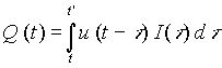 (6.22)
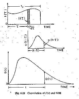
Fig. 6.21 Convolution of I (t ) and IUH
where t' = t when t < to
and t' = to when t ³ to
Equation (6.22) is called the convolution integral or Duhamel integral. The integral of Eq.(6.22) is essentially the same as the arithmetical computation of Eq. (6.5).
The main advantage of IUH is that it is independent of the duration of ERH and thus has one parameter less than a D-h unit hydrograph. This fact and the definition of IUH make it eminently suitable for theoretical analysis of rainfall excess-runoff relationship of a catchment. For a given catchment IUH, being independent of rainfall characteristics, is indicative of the catchment storage characteristics.
FLOODS
A flood is an unusually high stage in a river-normally the level at which the river overflows its banks and inundates the adjoining area. The damages caused by floods in terms of loss of life, property and economic loss due to disruption of economic activity are all too well-known. Crores of rupees are spent every year in flood control and flood forecasting. The hydrograph of extreme floods and stages corresponding to flood peaks provide valuable data for purposes of hydrologic design. Further, of the various characteristics of the flood hydrograph, probably the most important and widely used parameter is the flood peak. At a given location in a stream, flood peaks vary from year to year and their magnitude constitutes a hydrologic series which enable one to assign a frequency to a given flood-peak value. In the design of practically all hydraulic structures of the peak flow that can be expected with an assigned frequency (say 1 in 1 00 years) is of primary importance to adequately proportion the structure to accommodate its effect. The design of bridges, culvert waterways and spillways for dams and estimation of scour at a hydraulic structure are some examples wherein flood-peak values are required. To estimate the magnitude of a flood peak the following alternative methods are available:
• Rational method,
• Empirical method,
• Unit-hydrograph technique
• Flood-frequency studies.
The use of a particular method depends upon (i) the desired objective, (ii) the available data and (iii) the importance of the project. Further the rational formula is only applicable to small-size (< 50km²) catchments and the unit-hydrograph method is normally restricted to moderate-size catchments with areas less than 5000 km².
RATIONAL METHOD
Consider a rainfall of uniform intensity and very long duration occurring over a basin. The runoff rate gradually increases from zero to a constant value as indicated in Fig.7.1. The runoff increases as more and more flow from remote areas of the catchment reach the outlet. Designating the time taken for a drop of water from the farthest part of the catchment to
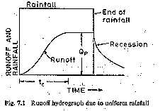
Fig. 7.1 Runoff hydrograph due to uniform rainfall
reach the outlet as the time of concentration, it is obvious that if the rainfall continues beyond tc, the runoit will be constant and at the peak value. The peak value of the runoff is given by Qp = C A i; for t ³ tc (7.1)
where C = coefficient of runoff = (runoff/rainfall), A = area of the catchment and i = intensity of rainfall. This is the basic equation of the rational method. Using the commonly used units, Eq. (7.1) is written for field application as
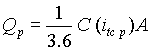 (7.2)
(7.2)
Where, Qp = peak discharge (m³/s)
C = coefficient of runoff
itcp = the mean intensity of precipitation (mm/h) for a duration equal to tc and
an exceedence probability P
A = drainage area in km²
The use of this method to compute Qp requires three parameters: tc, (ict p) and C.
EMPIRICAL FORMULAE
The empirical formulae u3ed for the estimation of the flood peak are essentially regional formulae based on statistical correlation of the observed peak and important catchment properties. To simplify the form of the equation, only a few of the many parameters affecting the flood peak are used. For example, almost all formulae use the catchment area as a parameter affecting the flood peak and most of them neglect the flood frequency as a parameter. In view of these, the empirical formula are applicable only in the region from which they were developed and when applied to other areas they can at best give approximate values.
Flood-Peak-Area Relationships
By far the simplest of the empirical relationships are those which relate the flood Peak to the drainage area. The maximum good discharge Qp from a catchment area A is given by these formulae as Qp = f(A)
UNIT-HYDROGRAPH
The unit-hydrograph technique described in the previous chapter used to predict the peak-flood hydrograph if the rainfall producing flood, infiltration characteristics of the catchment and the appropriate hydrograph are available. For design purposes, extreme rainfall situations are used to obtain the design storm, viz., the hyetograph of the rainfall excess causing extreme floods. The known or derived unit hydrograph of the catchment is then operated upon by the design storm to generate the desired flood hydrograph.
FLOOD-FREQUENCY STUDIES
Hydrologic processes such as floods are exceedingly complex natural events. They are resultants of a number of component parameters and are therefore very difficult to model analytically. For example, the floods in a catchment depend upon the characteristics of the catchment; rainfall and antecedent conditions, each one of these factors in turn depend upon a host of constituent parameters. This makes the estimation of the flood peak a very complex problem leading to many different approaches. The empirical formulae and unit-hydrograph methods presented in the previous sections are some of them. Another approach to the prediction of flood, lows, and also applicable to other hydrologic processes such as rainfall etc. is the statistical method of frequency analysis. The values of the annual maximum flood from a given catchment area for large number of successive years constitute a hydrologic data series called the annual series. The data are then arranged in decreasing order of magnitude and the probability P of each event being equalled to or exceeded (plotting position) is calculated by the plotting-position formula
 (7.11)
where m = order number of the event and N = total number of events in the data. The recurrence interval, T (also called the return period or frequency) is calculated as
 (7.12)
The relationship between T and the probability of occurrence of various events is the same as described in Sec. 2.10. Thus, for example, the probability of occurrence of the event r times in n successive years is given by
![]()
![]()
where q = 1-p
Consider, for example, a list of flood magnitudes of a river arranged in blending order is shown in Table 7.2. The length of the record is 50 years.
The last column shows the return Period T of various flood magnitude, Q. A plot of Q Vs T yields the probability distribution, for small return periods (i.e. for interpolation) or where limited extrapolation is required, a, simple best-fitting curve through plotted points can be used as the probability distribution. A logarithmic scale for T is often advantageous. However, when larger extrapolations of Tare involved, theoretical probability distributions have to be used. In frequency analysis of floods the usual problem is to predict extreme flood events. Towards this, specific extreme-value distributions are assumed and the required statistical parameters calculated from the available data. Using these the flood magnitude for a specific return period is estimated. Chow (1951) has shown that most frequency-distribution functions applicable in hydrologic studies can be expressed by the following equation known as the general equation of hydrologic frequency analysis:
XT, = ` x + K s #9; #9; #9; (7.13)
Where, XT = value of the variegate X of a random hydrologic series with a return period T, ` x = mean of the variegate, s = standard deviation of the variegate, K = frequency factor which depends upon the return period, T and the assumed frequency distribution. Some of the commonly used frequency distribution functions for the predication of extreme flood values are Gumbel's extreme-value distribution, Log-Pearson Type III distribution, and Log normal distribution.
PARTIAL-DURATION SERIES
In the annual hydrologic data series of floods, only one maximum value flood per year is selected as the data point. It is likely that in s catchments there are more than one independent floods in a year many of these may be of appreciably high magnitude. To enable all the large flood peaks to be considered for analysis, a flood magnitude than an arbitrary selected base value are included in the analysis. Such a data series is called partial-duration series.
In using the partial-duration series, it is necessary to establish that all events considered are independent. Hence the partial-duration adopted mostly for rainfall analysis where the conditions of independency of events are easy to establish. Its use in flood studies is rather rare. The recurrence interval of an event obtained by annual series (TA) an partial duration series (Tp) are related by
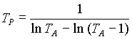 (7.28)
From this it can be seen that the difference between TA and Tp is significant for TA < 10 years and that for TA > 20, the difference is negligibly small.
REGIONAL FLOOD FREQUENCY ANALYSIS
When the available data at a catchment is too short to conduct frequency analysis, a regional analysis is adopted. In this a hydrologically homogeneous region from the statistically point of view is considered. Available long-time data from neighbouring catchments are tested for homogeneity and a group of stations satisfying the test are identified. This group of stations constitutes a region and all the station data of this region are pooled and analysed as a group to find the frequency characteristics of the region. The mean annual flood Qma, which corresponds to a recurrence interval of 2.33 years is used for nondimensionalising the results. The variation of Qma with drainage area and the variation of QT/Qma with T, where QT is the discharge for any Tare the basic plots prepared in this analysis.
LIMITATIONS OF FREQUENCY STUDIES
The flood-frequency analysis described in the previous sections is a direct means of estimating the desired flood based upon the available flood-flow data of the catchment. The results of the frequency analysis depend upon the length of data. The minimum number of years of record required to obtain satisfactory estimates depends upon the variability of data and hence on the physical and climatological characteristics of the basin. Generally a minimun of 30 years of data is considered as essential. Smaller lengths of records are also used when it is unavoidable. However, frequency analysis should not be adopted if the length of records is less than 10 years.
Flood-frequency studies are most reliable in climates that are uniform from year to year. In such cases a relatively short record gives a reliable picture of the frequency distribution. With increasing lengths of flood records, it affords a viable alternative method of flood-flow estimation in most cases.
DESIGN FLOOD
In the design of hydraulic structures it is not practical from economic considerations to provide for the safety of the structure and the system It the maximum-possible flood in the catchment. Small structures such as culverts and storm drainages can be designed for less severe floods as the consequences of a higher-than-design flood may not be very serious. It can cause temporary inconvenience like the disruption of traffic and very rarely severe property damage and loss of life. On the other hand, storage structures such as dams demand greater attention to the magnitude of floods used in the design. The failure of these structures causes large loss of life and great property damage on the down-stream of the structure.
From this it is apparent that the type, importance of the structure and economic development of the surrounding area dictate the design criteria for choosing the flood magnitude. This section highlights the procedures adopted in selecting the flood magnitude for the design of some hydraulic structures.
Design Flood
Flood adopted for the design of a structure.
Spillway Design Flood
Design flood used for the specific purpose of designing. the spillway of a storage structure. This term is frequently used to denote the maximum discharge that can be passed in a hydraulic structure without any damage or serious threat to the stability of the structure.
Standard Project Flood (SPF)
The flood that would result from a severe combination of meteorological and hydrological factors that are reasonably applicable to the region. Extremely rare combinations of factors are excluded.
Probable Maximum Flood (PMF)
The extreme flood that is Physically possible in a region as a result of severest combinations, including rare combinations of meteorological and hydrological factors.
The PMF is used in situations where the failure of the structure would result in loss of life and catastrophic damage and as such complete security from potential floods is sought. On the other hand, SPF is often used where the failure of a structure would cause less severe damages. Typically, the SPF is about 40 to 60% of the PMF for the same drainage basin. The criteria used for selecting the design flood for various hydraulic structures vary from one country to another.
DESIGN STORM
To estimate the design flood for a project by the use of a unit hydrograph, one needs the design storm. This can be the storm-producing probable maximum precipitation (PMP) for deriving PMF or a standard project (SPS) for SPF, calculations. The computations are performed by experienced hydrometeorologists by using meteorological data. Various methods ranging from highly sophisticated hydrometeorological methods to simple analysis of past rainfall data are in use depending on the availability of reliable relevant data and expertise.
The following is a brief outline of a procedure followed in India:
The duration of the critical rainfall is first selected. This will be the basin lag if the flood peak is of interest. If the flood volume is of prime interest, the duration of the longest storm experienced in the basin is selected. Past major storms in the region which conceivably could have occurred in the basin under study are selected. DAD analysis is performed and the enveloping curve representing maximum depth-duration relation for the study basin obtained.
Rainfall depths for convenient time intervals (e.g.6h) are scaled from the enveloping curve. These increments are to be arranged to get a critical sequence which produces the maximum flood peak when applied to the relevant unit hydrograph of the basin.
In critical sequence of rainfall increments can be obtained by trial and error. Alternatively, increments of precipitation are first arranged in a of relevant unit hydrograph ordinates such that
The design storm is then combined with hydrologic abstractions most conducive to high runoff, viz. low initial loss and lowest infiltration rate to get the hyetograph of rainfall excess to operate upon the unit hydrograph.
FLOOD ROUTING
The flood hydrograph discussed in Chap.6 is infact a wave. The stage and discharge hydrographs represent the passage of waves of river depth and discharge respectively. As this wave moves down the river, the shape of the wave gets modified due to various factors, such as channel storage, resistance, lateral addition or withdrawal of flows, etc. When a flood wave passes through a reservoir, its peak is attenuated and the time base is enlarged due to the effect of storage. Flood waves passing down a river have their peaks attenuated due to friction if there is no lateral inflow. The addition of lateral inflows can cause a reduction of attenuation or even amplification of a flood wave.
Flood routing is the technique of determining the flood hydrograph at a section of a river by utilizing the data of flood flow at one or more upstream sections. The hydrologic analysis of problems such as flood forecasting, flood protection, reservoir design and spillway design invariably include flood routing. In these applications two broad categories of routing can be recognised. These are Reservoir routing, and channel routing.
In reservoir routing the effect of a flood wave entering a reservoir is studied. Knowing the volume-elevation characteristic of the reservoir and the outflow-elevation relationship for the spillways and other outlet structures in the reservoir, the effect of a flood wave entering the reservoir is studied to predict the variations of reservoir elevation and outflow discharge with time. This form of reservoir routing is essential in the design of the capacity of spillways and other reservoir outlet structures and in the location and sizing of the capacity of reservoirs to meet specific requirements.
In channel routing the changes in the shape of a hydrograph as it travels down a channel is studied. By considering a channel reach and an input hydrograph at the upstream end, this form of routing aims to predict the flood hydrograph at various sections of the reach. Information on the flood-peak attenuation and the duration of high-water levels obtained by channel routing is of utmost importance in flood-forecasting operations and flood-protection works.
A variety of routing methods are available and they can be broadly classified into two categories as: (i) hydrologic routing and (ii) hydraulic routing. Hydrologic-routing methods employ essentially the equation of continuity. Hydraulic methods, on the other hand, employ the continuity equation together with the equation of motion of unsteady flow. The basic differential equations used in the hydraulic routing, known as St. Venant equations altord a better description of unsteady flow than hydrologic methods.
HYDROLOGIC CHANNEL ROUTING
In reservoir routing presented in the Previous sections, the storage was a unique function of the Outflow discharge S=f(Q). However, in channel routing the storage is a function of both Outflow and inflow discharges and hence a different routing method is needed. The flow in a river during a flood belongs to the category of gradually varied unsteady flow. surface in a channel reach is not only not parallel to the channel bottom but also varies with time (Fig.8.7). Considering a channel reach having a flood flow, the total volume in storage can be considered under two categories as Prism storage and wedge storage.
Prism Storage
It is the volume that would exist if uniform flow occurred at the downstream depth, i.e. the volume formed by an imaginary plane parallel to the channel bottom drawn at the outflow section water surface.
Wedge Storage
It is the wedge-like volume formed between the actual water surface profile and the top surface of the prism storage. At a fixed depth at a downstream section of a river reach the prism storage is constant while the wedge storage changes from a positive value at an advancing flood to a negative value during a receding flood.
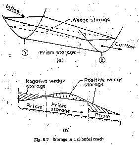
Fig. 8.7 Storage in a channel reach
The prism storage Sp is similar to a reservoir and can be expressed as a function of the outflow discharge, Sp =f(Q). The wedge storage Sw can be accounted for by expressing it as Sw = f(I). The total storage in the channel reach can then be expressed as
![]() (8.8)
(8.8)
where K and x are coefficients and m = a constant exponent. It has been found that the value of m varies from 0.6 for rectangular channels to a value of about 1.0 for natural channels.
Muskingum Equation
Using m = 1.0, Eq. (8.8) reduces to a linear relationship for S in terms of I and Q as
S= K [x I + (1-x) Q] (8.9)
and this relationship is known as the Muskingum equation. In this the parameter x is known as weighting factor. When x = 0, obviously the storage is a function discharge only and the Eq. (8.9) reduces to
S = K Q (8.10)
Such a storage is known as linear storage or linear reservoir. When x = 0.5 both the inflow and outflow are equally important in determining the storage. The coefficient K is known as storage-time constant and has the dimensions of time. It is approximately equal to the time of travel of a flood wave through the channel reach.
HYDRAULIC METHOD OF FLOOD ROUTING
The hydraulic method of flood routing is essentially a solution of the basic St Venant equations [Eq's(8.4) and (8.5)] . These equations are simultaneous, quasi-linear, first-order partial differential equations of the hyperbolic type and are not amenable to general analytical solutions. Only for highly simplified cases can one obtain the analytical solution of these equations. The development of modern, high-speed digital computers during the past two decades has given rise to the evolution of many sophisticated numerical techniques. The various numerical methods for solving St Venant equations can be broadly classified into two categories, Approximate methods and Complete numerical methods.
Approximate Methods
These are based on the equation of continuity only or on a drastically curtailed equation of motion. The hydrological method of storage routing and Muskingum channel routing discussed earlier belong to this category. Other methods in this category are diffusion analogy and kinematic Wave models.
Complete Numerical Methods
These are the essence of the hydraulic method of routing. In the direct method, the partial derivatives are replaced by finite differences and the resulting algebraic equations are then solved. In the method of characteristics (MOC) St Venant equations are converted into a pair of ordinary differential equations (i.e. characteristic forms) and then solved by finite difference techniques. In the finite element method (FEM) the system is divided into a number of elements and partial differential equations are integrated at the nodal points of the elements.
The numerical schemes are further classified into explicit and implicit methods. In the explicit method the algebraic equations are linear and the dependent variables are extracted explicitly at the end of each time step. In the implicit method the dependent variables occur implicitly and the equations are nonlinear. Each of these two methods has a host of finite-differencing schemes to choose from.
FLOOD CONTROL
The term "flood control" is commonly used to denote all the measures adopted to reduce damages to life and property by floods. As there is always a possibility, however remote it may be, of an extremely large flood occurring in a river the complete control of the flood to a level of zero loss is neither physically possible nor economically feasible. The flood control measures that are in use can be classified as:
1. Structural methods:
• Storage and detention reservoirs Levees (flood embankments),
• Channel Improvement, Flood ways (new channels), and
• Soil_Conservation
2. Non-structural methods: Flood plain zoning, #9; Flood warning and evacuation.
Storage Reservoirs
Storage reservoirs offer one of the most reliable and effective methods of control. Ideally, in this method, a part of the storage in the reservoir kept apart to absorb the incoming flood. Further, the stored water is deceased in a controlled way over an extended time so that downstream channels do not get flooded. Figure 8.13 shows an ideal operating plane of flood control reservoir. As most of the present-day storage reservoirs aye multipurpose commitments, the manipulation of reservoir levels to satisfy many conflicting demands is a very difficult and complicated task. It so happens that many storage reservoirs while reducing the floods and food damages do not always aim at achieving optimum benefits in the flood-control aspect. To achieve complete flood control in the entire length of a river, a large number of reservoirs at strategic locations in the catchment will be necessary.
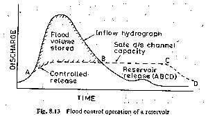
Fig. 8.13 Flood control operation of a reservoir
The Hirakud and Damodar Valley Corporation (DVC) reservoirs are examples of major reservoirs in the country which have specific volumes earmarked for flood absorption.
Detention Reservoirs
A detention reservoir consists of an obstruction to a river with an un-controlled outlet. These are essentially small structures and operate to reduce the flood peak by providing temporary storage and by restriction of the outflow rate. These structures are not common in India.
Levees
Levees, also known, as dikes or flood embankments are earthen banks constructed parallel to the course of the river to confine it to a fixed course and limited cross-sectional width. The heights of levees will be higher than the design flood level with sufficient free board. The confinement of the river to a fixed path frees large tracts land from inundation and consequent damage (Fig. 8.14).
Levees are one of the oldest and most common methods of flood protection works adopted in the world. Also, they are probably the cheapest of structural flood-control measures. While the protection offered by a levee against flood damage is obvious, what is not often appreciated is the potential damage in the event of a levee failure. The levees, being earth embankments require considerable care and maintenance. In the event of being overlapped, they fail and the damage caused can be enormous. In fact, the sense of protection offered by a levee encourages economic activity along the embankment and if the levee is overlapped the loss would be more than what would have been if there were no levees. Confinement of flood banks of a river by levees to a narrower space leads to higher flood levels for a given discharge. Further, if the bed level of the river also rises, as they do in agrading rivers, the top of the levees has to be raised at frequent time intervals to keep up its safety margin.
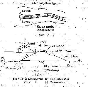
Fig. 8.14 A typical levee: (a) Plan (schematic)
The design of a levee is a major task in which costs and economic benefits have to be considered. The cross-section of a levee will have to be designed like an earth dam for complete safety against all kinds of saturation and drawdown possibilities. In many instances, especially in locations I where important structures and industries are to be protected, the water aside face of levees are protected by stone or concrete revetment. Regular maintenance and contingency arrangements to fight floods are absolutely necessary to keep the levees functional.
Masonry structures used to confine the river in a manner similar to levees are known as flood nails. These are used to protect important Structures against floods, especially where the land is at a premium.
Floodways
Floodways are natural channels into which a part of the flood will be diverted during high stages. A flood way can be a natural or man-made channel and its location is controlled essentially by the topography. Generally, wherever they are feasible, floodways offer an economical alternative to other structural flood-control measures. To reduce the level of the river Jhelum at Srinagari a supplementary channel has been constructed to act as a floodways with a capacity of 300 m3/s. This channel is located 5 km upstream of Srinagar city and has its outfall in lake Wullar.
Channel Improvement
The works under this category involve:
Widening or deepening of the channel to increase the cross-sectional area;
Reduction of the channel roughness, by clearing of vegetation from the channel perimeter;
Short-circuiting of meander loops by cutoff channels, leading to increased slopes.
All these three methods are essentially short-term measures and require continued maintenance.
Soil Conservation
Soil-conservation measures in the catchment when properly planned and effected lead to an all-round improvement in the catchment characteristics affecting abstractions. Increased infiltration, greater evapotranspiration and reduced soil erosion are some of its easily identifiable results. It is believed that while small and medium floods are reduced by soil-conservation measures, the magnitude of extreme floods is unlikely to be affected by these measures.
FLOOD FORECASTING
Forecasting of floods in advance enables a warning to be given to the people likely to be affected and further enables civil-defense measures to be organized. It thus forms a very important and relatively inexpensive nonstructural flood-control measure. However, it must be realised that a flood warning is meaningful if it is given sufficiently in advance. Also, erroneous warnings will cause the populace to loose faith in the system. Thus the dual requirements of reliability and advance notice are the essential ingredients of a flood-forecasting system. The flood forecasting techniques can be broadly divided into three categories:
Short-range forecasts,
Medium-range forecasts
Long-range forecasts.
Short-Range Forecasts
In this the river stages at successive stations on a river are correlated with hydrological parameters, such as precipitation area, antecedent precipitation index, and variation of the stage at the upstream base point during the travel time of a flood. This gives an advance warning of 12-40 h for floods. The flood forecasting currently being used for the metropolitan city of Delhi is based on this technique.
Medium-Range Forecasts
In this rainfall-runoff relationships are used to predict flood levels with a warning of 2-5 days. Coaxial graphical correlations of runoff with rainfall and other parameters like the time of the year, storm duration and antecedent wetness have been developed to a high stage of refinement by the US Weather Bureau.
Long-Range Forecasts
Using radars and meteorological satellite data, advance information about critical storm-producing weather systems, their rain potential and time of occurrence of the event are predicted well in advance.
FLOOD CONTROL IN INDIA
In India the Himalayan rivers account for nearly 60% of the flood damage in the country. Floods in these rivers occur during monsoon months and usually in the months of August or September. The damages caused by foods are very difficult to estimate and a figure of Rs. 10 billion as the annual flood damage in the country gives the right order of magnitude. It is estimated that annually on an average 40 Mha of land flooding and of this about 12 Mha have some kind of flood control measure. There are about 12,500 km of levees and about 25600 km drainage chennels affording protection from floods. About 60 to 80% of flood damages occur in the states of UP, Bihar, West Bengal, Assam and Orissa.
Flood forecasting is handled by CWC in close collaboration with the IMD, which lends meteorological data support. Nine flood Met offices both the aid of recording raingauges provide daily synoptic situations, actual rainfall amounts and rainfall forecasts to CWC. The CWC has 141 flood-forecasting stations situated on various basins to provide a forecasting service to a population of nearly 40 million.
A national programme for flood control was launched in 1954 and an amount of about 976 crores has been spent since then till the beginning of the Sixth Five-Year Plan. The Planning Commission has provided an outlay of 1045 crores in the sixth Five-Year Plan for flood control. These figures highlight the seriousness of the flood problem and the efforts made towards mitigating flood damages. The experience gained in the flood control measures in the country are embodied in the report of the Rashtriya Barh Ayog (RBA) (National Flood Commission) submitted in March 1980. This report, containing a large number of recommendations on all aspects of flood, control forms the basis for the evolution of the present national policy on floods.
GROUNDWATER
In the previous chapters various aspects of surface hydrology that deal with surface runoff have been discussed. Study of subsurface flow is equally important since about 22% of the world's fresh water resources exist in the form of groundwater. Further, the subsurface water forms a critical input for the sustenance of life and vegetation in and zones. Because of its importance as a significant source of water supply, various aspects of groundwater dealing with the exploration, development and utilization have been extensively studied by workers from different disciplines, such as geology, geophysics, geochemistry, agricultural engineering, fluid mechanics and civil engineering and excellent treatises are available.
FORMS OF SUBSURFACE WATER
Water in the soil mantle is called subsurface water and is considered in two zones (Fig. 9.1), Saturated zone and #9; Aeration zone.
Saturated Zone
This zone, also known as groundwater zone is the space in which all the pores of the soil are filled with water. The water table forms its upper limit and marks a free surface, i.e. a surface having atmospheric pressure.
Fig. 9.1 Classification of subsurface water
Zone of Aeration
In this zone the soil pores are only partially saturated with water. The space between the land surface and the water table marks the extent of this zone. Further, the zone of aeration has three subzones:
Soil Water Zone
This lies close to the ground surface in the major root band of the vegetation from which the water is lost to the atmosphere by evapotranspiration.
Capillary Fringe
In this the water is held by capillary action. This zone extends from the water table upwards to the limit of the capillary rise.
Intermediate Zone
This lies between the soil water zone and the capillary fringe. The thickness of the zone of aeration and its constituent subzones depend upon the soil texture and moisture content and vary from region to region. The soil moisture in the zone of aeration is of importance in agricultural practice and irrigation engineering. The present chapter is concerned only with the saturated zone.
All earth materials, from soils to rocks have pore spaces. Although these pores are completely saturated with water below the water table, from the groundwater utilization aspect only such material through which water moves easily and hence can be extracted with ease are significant. On this basis the saturated formations are classified into four categories: Aquifer Aquitard Aquiclude Aquifuge
Aquifer
An aquifer is a saturated formation of earth material which not only stores water but yields it in sufficient quantity. Thus an aquifer transmits water relatively easily due to its high permeability. Unconsolidated deposits of sand and gravel form good aquifers.
Aquitard
It is a formation through which only seepage is possible and thus the yield is insignificant compared to an aquifer. It is partly permeable.
Aquiclude
It is a geological formation which is essentially impermeable to the flow of water. It may be considered as closed to water movement even though it may contain large amounts of water due to its high porosity. Clay is an example of an aquiclude.
Aquifuge
It is a geological formation which is neither porous nor permeable. There are no interconnected openings and hence it cannot transmit water. Massive compact rock without any fractures is an aquifuge.
The definitions of aquifer, aquitard and aquiclude as above are relative. A formation which may be considered as an aquifer at a place where water is at a premium (e.g. and zones) may be classified as an aquitard or even aquiclude in an area where plenty of water is available.
The availability of groundwater from an aquifer at a place depends upon the rates of withdrawal and replenishment (recharge). Aquifers play the roles of both a transmission conduct and a storage. Aquifers are classified as unconfined aquifers and confined aquifers on the basis of their occurrence and field situation. An unconfined aquifer (also known as water table aquifer) is one in which a free surface, i.e. a water table exists (Fig. 9.2). Only the saturated zone of this aquifer is of importance in groundwater studies. Recharge of this aquifer takes place through infiltration of precipitation from the ground surface. A well driven into an unconfined aquifer will indicate a static water level corresponding to the water table level at that location.
A confined aquifer, also known as artesian aquifer, is an aquifer which is confined between two impervious beds such as aquicludes or aquifuges (Fig. 9.2). Recharge of this aquifer takes place only in the area where it is exposed at the ground surface. The water in the confined aquifer will be under pressure and hence the piezometric level will be much higher than the top level of the aquifer.
Fig. 9.2 Confined and unconfined acquirers
At some locations: the piezometric level can attain a level higher than the land surface and a well driven into the aquifer at such a location will flow freely without the aid of any pump. In fact, the term "artesian" is derived from the fact that a large number of such free-flow wells were found in Artois, a former province in north France. Instances of free-flowing wells having as much as a 50-m head at the ground surface are reported.
Water Table
A water table is the free water surface in an unconfined aquifer. The static level of a well penetrating an unconfined aquifer indicates the level of the water table at that point. The water table is constantly in motion adjusting its surface to achieve a balance between the recharge and outflow from the subsurface storage. Fluctuations in the water level in a dug well during various seasons of the year, lowering of the groundwater table in a region due to heavy pumping of the wells and the rise in the water table of an irrigated area with poor drainage, are some common examples of the fluctuation of the water table. In a general sense, the water table follows the topographic features of the surface. If the water table intersects the land surface the groundwater comes out to the surface in the form of springs or seepage. Sometimes a lens or localised patch of impervious stratum can occur inside an unconfined aquifer in such a way that it retains a water table above the general water table (Fig. 9.3). Such a water table retained around the impervious material is known as perched water table. Usually the perched water table is of limited extent and the yield from such a situation is very small. In groundwater exploration a perched water table is quite often confused with a general water table.
Fig. 9.3 Perched water table
AQUIFER PROPERTIES
The important properties of an aquifer are its capacity to release the water held in its pores and its ability to transmit the flow easily. These properties essentially depend upon the composition of the aquifer.
Porosity
The amount of pore space per unit volume of the aquifer material is called porosity. It is expressed as
 (9.1)
(9.1)
where n = porosity, Vv = volume of voids and Vo = volume of the porous medium, In an unconsolidated material the size distribution, packing and shape of particles determine the porosity. In hard rocks the porosity is dependent on the extent, spacing and the pattern of fracturing or on the nature of solution channels. In qualitative terms porosity greater than 20% is considered as large, between 5 to 20% as medium and less than 5% as small.
Specific Yield
While porosity gives a measure of the water-storage capability of a formation, not all the water held in the pores is available for extraction by pumping or draining by gravity. The pores hold back some water by molecular attraction and surface tension. The actual volume of water that can be extracted by the force of gravity from a unit volume of aquifer material is known as the specific yield, Sy. The fraction of water held back in the aquifer is known as specific retention, Sr. Thus porosity
n = Sy + Sr (9.2)
The representative values of porosity and specific yield of some common earth materials are given in Table 9.1.
TABLE 9.1 POROSITY AND SPECIFIC YIELD OF SELECTED FORMATIONS
|
Formation |
Porosity % |
Specific Yield % |
|
Lime stone |
1-10 |
0.5-5 |
|
Shale |
1-10 |
0.5-5 |
|
Sand Stone |
10-20 |
5-15 |
|
Gravel |
30-40 |
15-30 |
|
Sand |
35-40 |
10-30 |
|
Clay |
45-55 |
1-10 |
It is seen from Table 9.1 that although both clay and sand have high porosity the specific yield of clay is very small compared to that of sand.
GEOLOGICAL FORMATIONS AS AQUIFERS
The identification of a geologic formation as a Potential aquifer for ground Water-development is a specialized job requiring the services of a trained hydrogeologist. The geologic formations of importance for possible use as an aquifer can be broadly classified as unconsolidated deposits and consolidated rocks. Unconsolidated deposits of sand and gravel form the most important aquifers. They occur as fluvial alluvial deposits, abandoned channel sediments, coastal alluvium and as lake and glacial deposits. The yield is generally good and may be of the order of 50-100 m³/hr. In India, the Gangetic alluvium and the coastal alluvium in the states of Tamil Nadu and Andhra Pradesh are examples of good aquifers of this kind. Among consolidated rocks, rocks with primary porosity such as sandstones are generally good aquifers. The state of weathering of rocks and occurrence-of secondary openings such as joints and fractures enhance the yield. Normally, the yield from these aquifers is 1ess than that of alluvial deposits and typically may have a value of 20-50 m³/h. Sandstones of Kathiawar and Kutch areas of Gujarat and of Lathi region of Rajasthan are some examples.
Limestones contain numerous secondary openings in the form of cavities formed by the solution action of flowing subsurface water. Often these form highly productive aquifers. In Jodhpur district of Rajasthan, cavernous limestones of the Vindhyan system are providing very valuable ground-water for use in this arid zone.
The volcanic rock basalt has permeable zones in the form of vesicles, joints and fractures. Basaltic aquifers are reported to occur in confined as well as underunconfined conditions. In the Satpura range some aquifers of this kind give yields of about 20 m³/h.
Igneous and metamorphic rocks with considerable weathered and fractured horizons offer good potentialities as aquifers. Since weathered and fractured horizons are restricted in their thickness these aquifers have limited thickness. Also, the average permeability of these rocks decreases with depth. The yield is fairly low, being of the order of 5-10 m³/h. Aquifers of this kind are found in the hard rock areas of Karnataka, Tamil Nada, Andhra Pradesh and Bihar.
WELLS
Wells form the most important mode of groundwater extraction from an aquifer. While wells are used in a number of different applications, they find extensive use in water supply and irrigation engineering practice. Consider the water in an unconfined aquifer being pumped at a constant rate from a well. Prior to the pumping, the water level in the well indicates the static water table. A lowering of this water level takes place on pumping. If the aquifer is homogeneous and isotropic and the water table horizontal initially, due to the radial flow into the well through the aquifer the water table assumes a conical shape called cone of depression. The drop in the water table elevation at any point from its previous static level is called drawdown. The areal extent of the cone of depression is called area of influence and its radial extent radius of influence (Fig. 9.5). At constant rate of pumping, the drawdown curve develops gradually with time due to the withdrawal of water from storage. This phase is called unsteady flow as the water-table elevation at a given location near the well changes with time. On prolonged pumping, an equilibrium state is reached between the rate of pumping and the rate of inflow of groundwater from the outer edges of the zone of influence. The drawdown surface attains a constant position with respect to time when the well is known to operate under steady-flow conditions. As soon as the pumping is stopped, the depleted storage in the cone of depression is made good by groundwater inflow into the zone of influence. There is a gradual accumulation of storage till the original (static) level is reached. This stage is called recuperation or recovery and is an unsteady phenomenon. Recuperation time depends upon the aquifer characteristics.
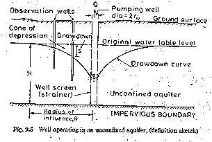
Fig.9.5 Well operating in an unconfined aquifer, (definition sketch)
Changes similar to the above take place due to a pumping well in a confined aquifer also, but with the difference that, it is the piezometric surface instead of the water table that undergoes drawdown with the development of the cone of depression. In confined aquifers with considerable piezometric head, the recovery into the well takes place at a very rapid rate.
GROUNDWATER BUDGET
The quantum of groundwater available in a basin is dependent on the inflows and discharges at various points. The interrelationship between inflows, outflows and accumulation is expressed by the water budget equation
å I D t - å Q D t = D S (9.39)
where,
å I D t = all forms of recharge and includes contribution by lakes, streams, canals, precipitation and artificial recharge, if any, in the basin
å Q D t = net discharge of groundwater from the basin and includes pumping, surface outflows, seepage into lakes and rivers and evapotranspiration
D S = change in the groundwater storage in the basin over a time D t
Considering a sufficiently long time interval, At of the order of a year, the capability of the groundwater storage to yield the desired demand and its consequences on the basis can be estimated. It is obvious that too large a withdrawal than what can be replenished naturally leads ultimately to the permanent lowering of the ground water table. This in turn leads to problems such as drying up of open wells and surface storages like swamps and ponds, change in the characteristics of vegetation that can be supported by the basin. Similarly, too much of recharge and scanty withdrawal or drainage leads to waterloggii3g and consequent decrease in the productivity of lands.
The maximum rate at which the withdrawal of groundwater in a basin can be carried without producing undesirable results is termed safe yield. This is a general term whose implication depends on the desired objective. The "undesirable" results include permanent lowering of the groundwater table or piezometric head, maximum drawdown exceeding a preset limit leading to inefficient operation of wells and salt-water encroachment in a coastal aquifer. Depending upon what undesirable effect is to be avoided, a safe yield for a basin can be identified.
ACID RAIN
Rain, which in the course of its history has combined with chemical elements or pollutants in the atmosphere and reaches the earth's surface as a weak acid solution.
ACIDITY OF WATER
Amount of acids, given as milli equivalents of a strong base per 1 litre of water, necessary to titrate the sample to a certain PH value.
ACTUAL EVAPOTRANSPIRATION
The real evapotranspiration occurring in a specific situation.
AFFLUENT
Watercourse flowing into a larger watercourse or into a lake.
ALBEDO
Ratio of reflected to incoming radiation, usually given in percent.
ALKALINITY OF WATER
Amount of cations balanced by weak acids, expressed as milli equivalents of neutralized hydrogen ions per litre of water.
ALLUVIAL PLAIN
Plain formed by the deposition of alluvial material eroded from areas of higher elevation.
ALLUVIAL STREAM
An alluvial stream is one whose bed is composed of unconsolidated silt, sand and gravel. The bed is constantly in motion and highly unstable.
ANEMOMETER
Instrument used for the measurement of wind speed and direction.
ANNUAL FLOOD
The highest peak discharge in a water year.
ANTECEDENT PRECIPITATION
The precipitation occurring during some period antecedent to the defined event or some part of the defined event.
ANTECEDENT PRECIPITATION INDEX
A weighed summation of daily precipitation amounts used as an index of soil moisture. The weight given to each day's precipitation is usually assumed to be an exponential or reciprocal function of time with the most recent precipitation receiving the greatest weight.
ANTICYCLONE
An area of relatively high pressure surrounded by closed isobars, the pressure gradient being directed from the center so that the wind blows spirally outward in a clockwise direction in the northern hemisphere, counter- clockwise in the southern hemisphere.
APPLIED HYDROLOGY
That branch of hydrology which refers to its applications to field connected with water resources development and management.
AQUICLUDE
It is a formation which may contain large volumes of water but does not permit its movement at rates sufficiently high for economical development e.g. clay and shale.
AQUIFER
It is a formation or a geological structure which has good permeability to supply sufficient quantity of water to a well or spring.
AQUIFUGE
It is a formation which has no interconnected openings and hence can not absorb or transmit water. It is neither porous nor permeable.
AQUITARD
It is a formation which has low to medium permeability which is not sufficient to be a source of water to flow on a regional scale from one aquifer to the other due to leakage. Formations having predominance of silt and clay along with kankar form aquitard. Behave as semi-confining layers.
AREA OF INFLUENCE
The areal extent of the cone of depression is called 'area of influence'.
AREA-ELEVATION-CAPACITY CURVE
Curves showing what part of the area of a watershed is situated above an indicated elevation and what is the capacity of watershed up to that elevation.
AREAL PRECIPITATION
Precipitation in a specific area expressed as the average depth of liquid water over this area.
AREA-VELOCITY METHOD
A method of measuring discharge at a section in a stream based on the continuity principle. Cross-sectional area of the stream is measured and velocity of flow is calculated using some type of instrument, say a current meter. Multiplication of area and velocity gives the discharge at that station.
ARID CLIMATE
A term applied to regions where precipitation is so deficient in quantity or occurs at such times that agriculture is impracticable without irrigation.
ARTESIAN AQUIFER
An artesian aquifer is overlain and underlain by confining layers such that water in these aquifers occurs under pressure, which is more than the atmospheric pressure.
ARTESIAN WELL
A well penetrating an artesian aquifer is called artesian well. If the water level rises above the bottom of the confining bed but remains below Ground surface, then it is called artesian well. If water rises above ground surface, then it is called flowing well.
ARTIFICIAL PRECIPITATION
It means causing precipitation artificially by the introduction of materials like solid carbon dioxide or silver iodide into a non-precipitating cloud. The experiments have not yet become of economic importance.
ARTIFICIAL RECHARGE
Artificial recharge may be defined as augmenting the natural replenishment of ground water storage by some method of construction, spreading of water or by artificially changing natural conditions.
ATMOMETER
Porous, porcelain spheres, cylinders or blocks commonly used by plant physiologists for measuring evaporation because evaporation from their surfaces is considered to be quite representative of that from plants.
AUXILIARY GAUGE
At those hydrometric stations where variable back-water occurs, it is necessary to utilize fall in a reach for the determination of discharge. An auxiliary gauge is installed some distance d/s with the same datum as that of the principal gauge.
AVAILABLE HEAD
Amount of fall in a stream which is available for hydroelectric power development.
AVALANCHE
A moving mass of debris, snow and ice sliding rapidly down a mountain slope.
AVERAGE ANNUAL FLOOD
A flood equal to the average of the annual floods during the period of record.
AVERAGE ANNUAL RAINFALL
Rainfall equal to the average of the annual rainfalls during the period of record.
BACKWASHING
Reversal of the flow of water under pressure, for example, in a well to free the screen or strainer and the adjacent aquifer of clogging material.
BACKWATER CURVE
Longitudinal profile of the water surface upstream in a stream where the water surface is raised by a natural or artificial obstruction.
BANK STORAGE
Water absorbed and stored in the banks of a stream, lake or reservoir and returned in whole or in part as the level of the surface water body falls.
BAROMETER
An instrument used for measuring pressure of the atmosphere.
BASE FLOW
The sustained or dry-weather flow of streams resulting from the outflow of permanent or perched ground water and from the draining of large lakes and swamps. Also water from glaciers, snow and all other possible sources not resulting from direct runoff.
BASIN
Area drained by a river is called basin of the river.
BASIN LAG
Actually basin lag (also known as lag time) is the time difference between the centroids of the input (rainfall excess) and the output (surface runoff). Physically, it represents the mean time of travel of water particles from all parts of the catchment to the outlet during a given storm.
BASIN RECHARGE
Basin recharge is the difference between precipitation and storm runoff. It is often being called loss because it represents loss to runoff, but the term loss is actually a misnomer from agricultural point of view.
BASIN RESPONSE
Manner in which a basin reacts to a meteorological event or sequence of events.
BED LOAD
Bed load may be defined as the load of bed material in the bed layer where suspension is impossible for fluid dynamic reasons. Sediment grains in the bed layer are not vertically supported by flow but rest on the bed almost continuously while sliding, rolling and jumping along.
BIFURCATION RATIO
The ratio of number of stream segments of a given order to the number of stream segments of the next higher order.
BRACKISH WATER
Water containing salts at a concentration significantly less than that of sea water. The concentration of total dissolved salts is usually in the range 100 10000 mg per liters.
BUBBLE GAUGE
In this gauge, compressed air or gas is made to bleed out at very small rate through an outlet placed at the bottom of the river. A pressure gauge measure gas pressure which is equal to the water column above the outlet. Small change in water surface elevation is felt as change in pressure.
CANOPY INTERCEPTION
Rainfall retained on standing vegetation and evaporated without dripping off or running down the stems or trunks.
CAPILLARY RISE
The maximum height to which water will rise due to capillary forces above the water table.
CAPILLARY WATER
Water held in the soil above the water table by capillary action.
CATCHMENT AREA
The drainage basin of a river is called its catchment area. The catchment area includes all points that lie above the elevation of the gauging station and within the topographic divide that separate adjacent watersheds.
CATCHMENT ORDER
A catchment order is described depending on the stream order at the outlet or gauging station. A stream of any order has two or more tributaries of the next lower order.
CHANNEL
A natural or artificial clearly distinguished waterway which periodically or continuously contains moving water or which forms a connecting link between two bodies of water.
CHANNEL DETENTION
Volume of water which can be temporarily stored in channels during flood periods.
CHANNEL PRECIPITATION
Precipitation which falls directly on the water surfaces of lakes and streams.
CHANNEL ROUTING
The routing of a flood wave in a stream when the only storage is the valley storage.
CHANNEL STORAGE
The quantity of water within the main channel.
CHEMICAL OXYGEN DEMAND
Mass concentration of oxygen equivalent to the amount of a specified oxidants consumed by dissolved or suspended matter when a water sample is treated with that oxidant under defined conditions.
CLASS-A PAN
It is an instrument used for estimation of evaporation. It is a standard par of 1210 mm diameter and 255 mm depth used by US Weather Bureau.
CLIMATE
The sum total of all atmospheric or meteorological influences principally temperature, moisture, wind, pressure and evaporation which combine to characterise a region and give it individuality by influencing the nature of its land forms, soil, vegetation and land use.
CLIMATE SHELTER
Climate station instruments that must be protected from condensation, precipitation and radiation are house in climate shelters or screens. The typical shelter is white, double-topped, with louvered sides to permit free circulation of air.
CLIMATIC CYCLE
Actual or supposed recurrences of such weather phenomena as wet and dry years, hot and cold years, at more or less regular intervals, in response to long range terrestrial and solar influences.
CLOUD BURST
Rain storm of high intensity and of a relatively short duration usually over a relatively small area.
CLOUD SEEDING
In cloud seeding, the clouds which contain appreciable amount of liquid water under colloidally stable conditions, are made colloidally unstable by the addition of dry ice, silver iodide or other chemical agents so that a certain part of this otherwise unavailable water will reach the ground as precipitation.
COLLUVIUM
Soil which is eroded from sloping land may become lodged at fence rows and vegetated areas or deposited below breaks in slopes in the form of colluvium.
COLORADO SUNKEN PAN
This pan, used to estimate evaporation is 920 mm square and 460 mm deep and buried into the ground within 100 mm of the top with the advantage that radiation and aerodynamic characteristics are similar to those of a lake.
COMPOUND HYDROGRAPH
The hydrograph of an intermittent storm when the flow on account of one substorm continues during the next substorm.
CONCENTRATION CURVE
The rising limb of a hydrograph which represents the increase in discharge due to gradual building up of storage in channels and over the catchment surface.
CONCENTRIC RING INFILTROMETER
This is an instrument used for the measurement of infiltration. It consists of two concentric rings which are inserted into the ground and water is maintained on the soil surface to a common fixed level.
CONCEPTUAL HYDROLOGICAL MODEL
Simplified mathematical representation of some or all of the processes in the hydrological cycle by a set of hydrological concepts expressed in mathematical notations and linked together in a time and space sequence corresponding to that occurring in nature. Hydrological conceptual models are used for simulation of the behaviour of the basin.
CONDENSATION NUCLEI
Condensation of water vapour into cloud droplets takes place on certain hygroscopic particles which are commonly called condensation nuclei.
CONE OF DEPRESSION
A downward curve showing the variation of draw down with distance from the well describes a conic shape in three dimensions called cone of depression.
CONFIDENCE LIMITS
Values which form the lower and upper limits to the confidence interval.
CONFINED AQUIFER
A confined aquifer, also known as artesian or pressure aquifer, is an aquifer which is confined between two impervious beds such as aquicludes or aquifuges and in which groundwater is confined under pressure greater than atmosphere.
CONFLUENCE
Joining, or the place of junction, of two or more streams.
CONJUNCTIVE USE
Conjunctive use involves the coordinated and planned operation of both surface water and ground water resources to meet water requirements in a manner whereby water is conserved. The basic difference between the usual surface water development with it's associated ground water development and a conjunctive operation of surface water and ground water resource is that the separate firm yields of the former can be replaced by larger and more economic joint, yields of the later.
CONSUMPTIVE USE
The quantity of water used by vegetative growth of a given area in transpiration or building of plant tissue and that evaporated from the soil or from intercepted precipitation on the area in any specified time. It is expressed in water depth unit or depth-area units per unit area and for specified periods, such as days, months and seasons.
CONTAMINATION
Introduction of any undesirable substance, normally not present, in water, e.g. micro-organisms, chemicals, waste or sewage, which renders the water unfit for its intended use.
CONTROL SECTION
Reach of a stream channel in which there exists a unique stage- discharge relationship.
CONVECTIVE PRECIPITATION
Precipitation resulting from the upward movement of air that is warmer than its surrounding. It is generally of a showery nature with rapid changes of intensities.
CORRELATION COEFFICIENT
Measure of the inter-dependence between two variates.
COVARIANCE
First product moment of two variates about their mean values.
CREST SEGMENT
It is that part of the hydrograph which contains the peak flow. Peak flow occurs when the runoff from various parts of the catchment simultaneously contribute the maximum amount of flow at the basin outlet.
CREST STAGE INDICATOR
This indicator is used to delineate the peak stage of a flood at points other than at a hydrometric station. Such data are valuable in the establishment of flood profiles.
CRITICAL STORM PERIOD
The duration of that storm which causes the greatest peak at a station in a drainage basin.
CROP COEFFICIENT
It is an empirical coefficient used in Blaney-Criddle formula for calculating the potential evapotranspiration for a particular crop. It is different for different crops.
CROSS SECTION
Section of a stream at right angles to the main (average) direction of flow.
CRYOLOGY
The science of ice in all its forms such as snow, ice and hall.
CUP-TYPE CURRENT METER
Current meter whose rotor is composed of a wheel fitted with cups and turning on a vertical axis.
CURRENT METER
It is the most commonly used instrument in hydrometry for measuring the velocity at a point in the flow cross-section of a river.
CYCLONIC PRECIPITATION
The precipitation associated with the passage of depressions of cyclones.
DAM
Barrier constructed across a valley for impounding water or creating a reservoir.
DARCY'S LAW
It states that the rate of flow per unit area of an aquifer is proportional to the gradient of the potential head measured in the direction of flow.
DATA BASE
Comprehensive set of related data files for a specific application, usually on a direct access storage device.
DATA PROCESSING
Handling of observational data until they are in a form ready to be used for a specific purpose.
DEAD STORAGE
Storage volume which can not be released under normal conditions.
DEAD WATER
Water in a state of slow or no circulation, usually leading to an oxygen deficit.
DEEP PERCOLATION
Water which percolates below the root zone and towards a deeper water table.
DEGREE DAY
It is a unit expressing the amount of heat in term of the departure of one degree per day in the daily mean temperature from an adopted reference temperature. The number of degree days for an individual day is the actual departure of the mean temperature from the standard. Standard temperature is usually taken as 0 C to 32 F.
DENSITY CURRENT
It is defined as the gravitational flow of one fluid under another fluid of approximately equal density. Density currents thus separate the turbid water from the clear water and make the turbid water flow along the river bottom in the vicinity of the dam.
DEPENDABLE FLOW
In the flow-duration curve, the ordinate Qp at any percentage probability Pp represents the flow magnitude in an average year that can be expected to be equalled or exceeded Pp % of time is called Pp % dependable flow. For perennial streams, Q is a finite value while for ephemeral stream Q is zero.
DEPLETION CURVE
The depletion curve extends from the point of inflection at the end of the crest segment to the commencement of natural groundwater flow in a hydrograph. It represents the withdrawal of water from the storage built up in the basin during earlier phases of the storm.
DEPRESSION STORAGE
Also called pocket storage, the volume of water usually expressed as depth on the drainage area which is required to fill natural depressions, large or small, to their overflow levels.
DEPTH OF RUNOFF
The total runoff from a drainage area or basin, divided by the area, expressed in either units of depth or units of volume per unit area of the basin.
DEPTH-AREA RELATIONSHIP
It is a relation which is expressed between progressively decreasing average depth of rainfall of a given duration over a progressively increasing area from centre of maximum precipitation of a storm outward to its edges in an exponential fashion.
DEPTH-AREA-DURATION CURVE
A curve which graphically indicates the precipitation amounts for various areas and durations for a particular rainstorm.
DETENTION RESERVOIR
Flood-control reservoir with uncontrolled outlets.
DETERMINISTIC HYDROLOGY
Method of analysis of hydrological processes, using a deterministic approach to investigate the responses of hydrological systems in terms of various parameters.
DEW
Deposit of water drops on objects at or near the ground, produced by the condensation of water vapour from the surrounding clear air.
DIFFUSION WELL
Recharge well that is sunk only into the unsaturated zone distinguished from an injection well.
DISCHARGE COEFFICIENT
Ratio of the observed or actual discharge to the theoretically computed discharge.
DOWNSTREAM
In the direction of the current in a river or stream.
DRAINAGE
Removal of surface water or groundwater from a given area by gravity or by pumping.
DRAINAGE BASIN
The area from which a lake, stream or waterway and reservoir receives surface flow which originates as precipitation.
DRAINAGE COEFFICIENT
Drainage coefficient is the water depth drained from an area in one day. These coefficients enable the designer to compare various drainage methods.
DRAINAGE DENSITY
It is defined as the ratio of the total channel length to the total drainage area. A large drainage density creates situation conducive for quick disposal of runoff which is reflected in pronounced peaked discharge.
DRAWDOWN
The drawdown at a given point is the distance by which water level is lowered.
DRAWDOWN CURVE
A drawdown curve shows the variation of drawdown with distance from the well. In three dimensions, the drawdown curve describes a conic shape known as the cone of depression.
DRIZZLE
A fine sprinkle of numerous water droplets of size less than 0.5 mm and intensity less than 1mm/h. The drops are so small that they appear to float in the air.
DROUGHT
In general an extended period of dry weather or a period of deficient rainfall that may extend over an indefinite number of days. Without any set quantitative standard by which to determine the degree of deficiency needed to constitute a drought. Qualitatively, it may be defined by its effects, as a dry period sufficient in length and severity to cause at least partial crop failure.
DROUGHT INDEX
Computed value which is related to some of the cumulative effects of a prolonged and abnormal moisture deficiency. An index of hydrological drought corresponding to levels below the mean in streams, lakes, reservoirs and the like. However, an index is agricultural drought must relate to the cumulative effects of either an absolute or an abnormal transpiration deficit.
DRY YEAR
Year of drought in which precipitation or streamflow is significantly less than normal.
DRY-WEATHER FLOW
The flow of water in a stream during the non-rainy season. It is primarily made of water which seeps from the ground. However, water supplied by snowmelt or regulated water released from a storage also become a part of it.
DURATION CURVE
A graph representing the time during which the value of a given parameter e.g. water level, piezometric head, discharge, concentration of dissolved solids, is equalled or exceeded regardless of continuity in time.
ECHO-DEPTH RECORDER
An instrument by which the depth of water is determined by measuring the time taken by a sound signal to travel to the bottom and return.
EFFECTIVE RAINFALL
Part of the rain that appears as runoff in the stream.
EFFLUENT STREAM
A stream or stretch of stream which receives water from groundwater in the zone of saturation. The water surface of such a stream stands at a lower level than the water table or piezometric surface of the ground water body from which it receives water. Also a stream flowing out of another stream or out of a lake.
ELECTROMAGNETIC FLOWMETER
It is an instrument for measuring discharge in a stream. It is based on the principle that an e.m.f. is induced in the conductor (water in the present case) when it cuts a normal magnetic field.
ELONGATION RATIO
It is defined as the ratio of diameter of a circle of the same area as the basin to the maximum basin length. This ratio runs between 0.6 to 1.0 over a wide variety of climatic and geologic types.
EMERGENCY SPILLWAY
Auxiliary spillway used in the event of floods exceeding the capacity of the main spillway.
EMPIRICAL FLOOD FORMULA
Formula expressing peak discharge as a function of catchment area and other factors.
ENERGY BUDGET METHOD
It is an analytical method for the determination of evaporation. It is a measurement of continuity of flow of energy. Energy available for evaporation is determined by considering the incoming energy, outgoing energy and energy stored in the water body over a known time interval.
ENGINEERING HYDROLOGY
That branch of applied hydrology which deals with hydrological information intended for engineering applications, e.g. planning, designing, operating and maintaining engineering measures and structures.
ENVELOP CURVES
(a) A smooth curve which envelops all the plotted points representing maximum recorded
flood peaks and volumes for hydrometeorologically comparable areas.
(b) A smooth curve covering either all peak values or all trough values of certain quantities
e.g. rainfall, runoff etc. plotted against other factors such as area and time. In general,
none of the peak values goes above the curve in former case, called the "maximum
envelop" and non of the minimum points fall below in the later case called the "minimum
envelop".
EPHEMERAL STREAM
A stream or a portion of a stream which flows only in direct response to precipitation.
EQUILIBRIUM EQUATION
Equilibrium equation is used to determine the hydraulic conductivity or the transmissivity of a confined aquifer from a pumped well by measuring draw downs in two observation wells at different distances from a well pumped at constant rate.
EROSION
It is defined as the wearing away of land by water, wind, ice or gravity.
EUTROPHIC LAKE
Lake characterized by a great amount of nutrients and biogenic matters and by highly developed phytoplankton is summer.
EVAPORATION
The process by which water is changed from the liquid state to the gaseous state below the boiling point through the transfer of heat energy.
EVAPORATION OPPORTUNITY
Ratio of actual rate of evaporation from land or water surface in contact with the atmosphere to the potential rate of evaporation under existing atmospheric conditions.
EVAPORATION PAN
An experimental tank used to determine the amount of evaporation from the surface of water under measured or observed climatic conditions.
EVAPOTRANSPIRATION
An instrument for measuring evaporation.
EVAPOTRANSPIRATION
It is the process by which water moves from the soil to the atmosphere. It consists of transpiration, the movement of water through the plant to the atmosphere & evaporation, the movement of water vapour from soil and vegetative surfaces. Thus the entire surface as well as subsurface water which is released from a basin into the atmosphere by process of evaporation and transpiration is generally known as evapotranspiration.
EXCEEDENCE INTERVAL
The exceedence interval is defined as the average number of years between the occurrence of an event and a greater event.
EXPERIMENTAL BASIN
Basin in which natural conditions are deliberately modified and in which the effects of these modifications on the hydrological cycle are studied.
EXTREME RAINFALL
Amount of precipitation that is the physical upper limit for a given duration over a particular basin.
EXTREME VALUE DISTRIBUTION
Fisher Tippet Type I External distribution applied by Gumbel to the annual maximum flood series and by others to rainfall series.
FAIR-WEATHER RUNOFF
Also called base flow, it is composed of ground water runoff and delayed subsurface runoff.
FIELD CAPACITY
The amount of water held in the soil after the excess gravitational water has drained away and after the rate of downward movement of water has materially decreased. Essentially the same as 'specific retention', a more general term used in studies of ground water which covers all types of strata. Furthermore, field capacity is usually expressed as a percentage of weight while specific retention is generally given as percentage by volume.
FIELD EFFICIENCY
The percentage of the total volume of water delivered to the field that is finally consumed by evapotranspiration.
FIRN LINE
Boundary which, at the Earth's surface, separates zone of accumulation of a glacier from the zone of ablation.
FLASH FLOOD
A flood of short duration and abrupt rise with a relatively high peak rate of flow, usually resulting form a high intensity of rainfall.
FLOAT GAUGE
This is most common type of automatic float operated stage recorder. Float operating in a stilling well is balanced by means of a counter weight over the pulley of a recorder. Displacement of float is traversed on a chart continuously and stage versus time plot is made.
FLOATING PAN
It is US Geological Survey evaporation pan set afloat in a lake with a view to simulate the characteristics of a large body of water. Water level in the pan is kept at the same level as the lake, leaving a ring of 75 mm.
FLOOD
The flow pattern in a stream, constituting a distinct progressive rise culminating in a peak or summit together with the recession that follows the crest.
FLOOD ABATEMENT
Any measure taken outside of stream channel with the effect of educing the crest of flood flows or changing the debris load for a flood event.
FLOOD ABSORPTION
The increase in storage of water in a reservoir, lake, valley or channel resulting in a reduction of streamflow.
FLOOD CONTROL
Flood control means flood damage prevention or reduction together with the protection of economic development and protection of life.
FLOOD DAMAGE
The destruction or impairment, partial or complete, of human and animal lives, property, goods, services, flora and fauna or of health etc., resulting from the action of floods water and the silt and debris they carry. It includes direct and indirect losses.
FLOOD DISCHARGE
It is the discharge passing at a particular site during a flood event.
FLOOD FORECASTING
Prediction of stage, discharge, time of occurrence and duration of a flood, especially of peak discharge, at a specified point on a stream resulting from precipitation or snowmelt so that people could be warned well in advance and life and movable goods could be saved to a large extent.
FLOOD FREQUENCY
(a) The number of times a flood of a given magnitude is likely to be equaled or exceeded over
a period of years on the average.
(b) The number of years in which a flood of a given magnitude is likely to be equaled or
exceeded once on the average over a period of years.
FLOOD MARKS
The trace of any kind left on the banks or flood plain by a flood which may be used, after the flood, to determine the highest level attained by the water surface during the flood.
FLOOD PLAIN
Land adjoining the channel which is inundated only during floods.
FLOOD PROOFING
Combination of emergency equation and structural adjustments for modifying a given property and thus reducing flood losses.
FLOOD ROUTING
The process of determining progressively the timing and shape of a flood wave at successive points along a river.
FLOOD SERIES
A List of flood events which occurred during a specified period of time.
FLOOD STAGE
The elevation of water surface during a flood relative to a datum, local or national.
FLOOD WAY
The channel of a river or stream and those portions of the flood plains adjoining the channel, which are required to carry and discharge the flood water.
FLOW DURATION CURVE
Curve showing the percentage of time during which the flow of a stream is equal to or greater than given amounts, regardless of chronological order.
FLOW METER
It is an instrument used for measuring the rate of flow in a conduit or open channel.
FLOW-MASS CURVE
A graph of the cumulative values of discharge of runoff, generally as ordinate, plotted against time as abscissa. The curve has many useful applications such as the determination of reservoir capacity, operations procedure and flood routing.
FOREST HYDROLOGY
It is the science of water related phenomena that are influenced by forest cover. It is an interdisciplinary science, the union of forestry and hydrology.
FORMATION LOSS
It is the head drop required to cause laminar flow through the porous media.
FREEBOARD
Vertical distance between the normal maximum level of the surface of liquid in a conduit, reservoir, tank, canal, etc. and the top of the sides of the retaining structure.
FREQUENCY ANALYSIS
Procedure involved in interpreting a past record of hydrological events in terms of future probabilities of occurrence, e.g. estimates of frequencies of floods, droughts, storage, rainfall, water quality, waves.
FREQUENCY DISTRIBUTION
Specification of the way in which the frequencies of members of a population are distributed according to the values of the variates which they exhibit (DST).
FRESH WATER
Water neither salty nor bitter to the taste and in general, chemically suitable for human consumption (having a low content in dissolved solids).
FRONTAL PRECIPITATION
Precipitation caused by the expansion of air on ascent along or near a frontal surface.
FROST
A light feathery deposit of ice caused by condensation of water vapour directly in the crystalline form, on terrestrial objects whose temperature is below freezing, the process being the same by which dew is formed, except that the later occurs only when the temperature of the bedewed object is above freezing.
GAINING STREAM
Stream fed by groundwater.
GAUGE
An instrument used for measuring depth of water.
GAUGING SITE
Location on a stream where measurements of water level and discharge are regularly made.
GEOHYDROLOGY
Branch of hydrology related to subsurface and subterranean water.
GLACIER
Body of land ice formed from recrystallised snow accumulated on the ground; may form where annual accretion of snow is greater than ablation by runoff and evaporation. There are two broad classes
(a) Ice streams which form in mountain valleys and move downslope under gravity.
(b) Ice cap which cover large land masses and spread out radially because of great pressures
built up by their weight.
GLACIOMETER
An instrument used for measuring glacial motion.
GRAVITATIONAL WATER
Water in the unsaturated zone which moves under the influence of gravity.
GLAZE
Also called freezing rain, it is reported when rain falls into a cold layer of air and freezes when it strikes objects on the ground.
GROUND WATER
Water in a saturated zone of geologic stratum.
GROUND WATER BASIN
It may be defined as a hydrogeologic unit containing one large aquifer or several connected and interrelated aquifers. It implies an area containing a groundwater reservoir capable of furnishing a substantial water supply.
GROUNDWATER RECESSION
Decreasing rate of groundwater discharge to surface water bodies during periods of no recharge, connected to the depletion of ground water storage, and expressed by groundwater recessive curve.
GROUNDWATER RECHARGE
Process by which water is added from outside to the zone of saturation of an aquifer, either directly into a formation, or indirectly by way another formation.
GROUND WATER RUNOFF
That part of the runoff which consists of water that has passed into the earth and has entered the zone of saturation and has later been discharged into a water body.
GULLY
A channel or miniature valley formed as a result of erosion and caused by concentrated but intermittent flow of water usually during or immediately after heavy rains. The channel is deep enough to interior with tillage operations. Gully may be dendritic or branching or linear (long, narrow and of uniform width). Gully may be U, V or W shaped.
GUMBEL'S DISTRIBUTION
It is one of the most widely used probability distribution functions for extreme values in hydrologic and meteorologic studies for prediction of flood peaks, maximum rainfall, maximum wind speed etc.
HAIL
Small, roughly spherical lumps of approximately concentric shells of clear ice and compact snow usually ranging from 5 to 10 mm or more in diameter which fall either separately or agglomerated into larger irregular lumps precipitated during thunder storms.
HARDNESS OF WATER
That property of water, due mainly to bicarbonates, chlorides anulphates of calcium and magnesium, which prevents the production of abundant lather with soap.
HEAD LOSS
Decrease of total head, expressed in units of height, due to energy dissipation.
HEADWATERS
Streams from the sources of a river.
HEAVY WATER
Water enriched in water molecules containing heavier (stable and radioactive) isotopes of hydrogen (Deuterium, Tritium) and Oxygen 18.
HISTOGRAM
Univariate frequency diagram with rectangles proportional in area to the class frequency, erected on a horizontal axis with width equal to the class interval.
HISTORICAL DATA
Hydrological and Meteorological data of events which occurred in the past. Data is collected from natural phenomena that can be observed only once and then will not occur again.
HURRICANE
These are very intense low pressure systems with winds in excess of 75 m.p.h. It is an intense cyclone of tropical origin and of relatively small horizontal dimensions (110-300 miles). Storms of this type are called cyclones in India and typhoons in the far east. Hurricanes form where sea surface temperature is above 27 C in general; hurricanes are accompanied by torrential rains.
HYDRAULIC CONDUCTIVITY
It is a constant that serves as a measure of permeability of the porous medium. A medium has a unit hydraulic conductivity if it will transmit in unit time a unit volume of ground water at the prevailing kinematic viscosity through a cross section of unit area measured at right angles to the direction of flow, under a unit hydraulic gradient.
HYDRAULIC GRADIENT
(1) In a closed conduit the slope of the hydraulic grade line.
(2) In open channels: the slope of the water surface.
(3) In porous media: measure of the decrease in head per unit distance in the direction of flow.
HYDROGEOLOGY
That branch of geology relating to effect of water on earth.
HYDROGRAPH
A graph showing the stage, volume of flow, velocity, sediment concentration or sediment discharge or some other feature of flowing water with respect to time at a given place. For example, a graph showing the discharge of a stream as ordinate against time as abscissa is called a discharge hydrograph.
HYDROLOGIC CYCLE
A phenomena relating to circulation of water from the sea, through the atmosphere to the land, and thence, often with many delays, back to the sea or ocean through various stages and processes, for example, precipitation, interception, runoff, infiltration, percolation, ground water storage, evaporation and transpiration. Also the many short circuits of the water that is returned to the atmosphere without reaching the sea.
HYDROLOGIC EQUATION
The water inventory equation (inflow = o0utflow + change in storage) which expresses the basic principle that during a given time interval the total inflow to an area must equal the total outflow plus the net change in storage.
HYDROLOGIC FAILURE
Failures due to improper assessment of hydrological factors such as overtopping and consequent failure of an earthen dam due to inadequate spillway capacity, failure of bridges and culverts due to excess flood flow, inability of a large reservoir to fill up due to overestimation of stream flow etc.
HYDROLOGIC NETWORK
It is a network of stations for measuring hydrologic variables such as rainfall and river stage stations. Adequacy of hydrologic network is dependent upon the character of the drainage basin and the critical need of the regulating system.
HYDROMETEOROLOGY
Study of the atmospheric and land phases of the hydrological cycle, with emphasis on the interrelationships involved.
HYDROLOGY
The applied science concerned with the water of the earth in all its stages their occurrences, distribution and circulation through the unending hydrologic cycle of precipitation, runoff, streamflow, infiltration, storage, evaporation and reprecipitation. It is concerned with the physical, chemical and physiological reactions of water with the rest of the earth and its relation to the life of the earth.
HYDROMETRY
The measurement and analysis of the flow of water as well as the measurement of the specific gravity of water or suspensions of finely divided solids in water.
HYDROMETRY STATION
These are the stations where measurement of discharge in a stream is made at particular points. These must be sited adequately in the catchment area so that the water potential of the area can be assessed as accurately as possible.
HYETOGRAPH
A bar graph of average rainfall, rainfall excess rates or volumes over specified areas during successive units of time during a storm.
HYSTERESIS
The phenomenon that soil moisture tension at a given moisture content depends on the past history of wetting and drying cycles (of soil moisture). The variability of the stage-discharge relation at a gauging station subject to variable slope where, for the same gauge height, the discharge on the rising stage is greater than on the falling stage.
ISI STANDARD PAN
This pan evaporimeter specified by IS, also known as modified class A pan, consists of a pan 1220 mm in diameter, 255 mm deep and made of copper sheet 0.9 mm thick. The top is fully covered with a hexagonal wire mesh to protect water from birds.
ICE
Solid form of water in nature formed by the freezing of water, the condensation of atmospheric water vapour directly into crystals, the compaction of snow with or without the motion of a glacier or the impregnation of porous snow masses with water which subsequently freezes.
ICE CAP
Perennial cover of ice and snow over an extensive are a of land or sea.
INDUCED RECHARGE
It is water entering the ground from a surface water source as a result of withdrawal of ground water adjacent to the source. Induced recharge can furnish water free of organic matter and pathogenic bacteria.
INFILTRATION
The entrance of water into the soil or other porous material through the interstices or pores of a soil or other porous medium.
INFILTRATION CAPACITY
Maximum rate at which specified soil in given condition can absorb water.
INFILTRATION CAPACITY CURVE
A curve showing what the infiltration rate would be at any period during a specified storm if the rainfall intensity were to equal or exceed the capacity at any instant.
INFILTRATION INDEX
Infiltration index, in general, expresses infiltration at an average rate throughout the storm.
INFILTROMETER
A device by which the rate and amount of water infiltrating into the soil is determined.
INFLECTION POINT
It is a point on the hydrograph which represents start of withdrawal of water from the storage built up in the basin during the earlier phases of the hydrograph. It is the starting point of the recession limb and end point of crest segment. Point of inflection represents the condition of maximum storage.
INFLUENT STREAM
A stream or stretch of stream which contributes water to the zone of saturation. The water surface of such stream stands at a highest level than the water table or piezometric surface of the ground water body to which it contributes water.
INITIAL ABSTRACTION
Maximum amount of rainfall that can be absorbed under specific conditions without producing runoff. Also referred to as initial losses, it is sum of interception and depression storage.
INITIAL DETENTION
That part of precipitation which does not appear either as infiltration or as surface runoff during period of precipitation or immediately thereafter, includes interception by vegetal cover, depression storage and evaporation during precipitation, does not include surface detention.
INSTANTANEOUS UNIT HYDROGRAPH
When the unit duration of the rainfall excess is infinitesimally small, the resulting hydrograph is known as instantaneous unit hydrograph.
INTENSITY-DURATION-FREQUENCY CURVE
The intensity of storms decreases with the increase in storage duration. Further a storm of any given duration will have a larger intensity if its return period is large. The curves showing the interdependence between the intensity, duration and return period are commonly referred to as intensity duration frequency curves.
INTERCEPTION
The process by which precipitation is caught and held by foliage twigs and branches of the trees, shrubs and other vegetation, and lost by evaporation, never reaching the surface of the ground.
INTERCEPTOMETER
Throughfall gauges are called interceptometers, evidently because of their function in estimating canopy interception.
INTERFLOW
A part of the precipitation that infilters into the ground moves laterally through upper crusts of the soil and returns to the surface at some location away from the point of entry into the soil. This component of runoff is known as interflow. The amount of interflow depends on the geological conditions of the catchment.
INTERMITTENT STREAM
Stream which flows during a season. It has limited contribution from the ground water. During the wet season, water table is above the stream bed and there is contribution of base flow to the stream flow. During dry season, water table drops below stream bed and stream dries out.
IRRIGATION REQUIREMENT
Quantity of water, exclusive of precipitation, that is required for optimal crop production.
ISOCHRONE
It is a line on a map of a catchment joining points having equal time of travel to the outlet of the catchment.
ISOHYET
A line drawn on a map passing through places having equal amount of rainfall recorded during the same period at these places (these lines are drawn after giving consideration to the topography of the region).
ISOPLETH
Lines on a map through places having equal depths of evapotranspiration.
ISOTHERM
Lines joining points of equal temperatures.
JUVENILE WATER
It is water derived from magma or molten mass of igneous rocks during their crystallisation or from lava flows in the form of stream. It is water that has come to the earth surface from great depths for the first time.
KARSTIC RIVER
River which originates from a karstic spring or flows in a karstic region that is, in a region having carbonaceous rocks as CaCo3.
LAG TIME
It is the time interval from the centre of mass of rainfall to the centre of mass of hydrograph.
LAKE
An extensive sheet of water, bounded by land, in a hollow of the earth surface. It is an inland body of water which is formed more due to glacial erosion than due to any other agency.
LAND PAN
It is a pan placed on the ground for the purpose of measuring evaporation.
LARGE WATERSHED
A large watershed is one in which the effect of channel flow or basin storage is dominating rather than the effect of overland flow. It has very less sensitivity to high intensity rainfall of short duration.
LATERAL INFLOW
Inflow of water to a river, lake or reservoir along any reach from the part of the catchment adjacent to the reach.
LEACHING REQUIREMENT
Water required for the removal of salts from the upper soil by relatively salt-free water.
LEAKY AQUIFER
Aquifers which are overlain or underlain by semi-permeable strata are referred to as leaky aquifers. Such aquifers are confined in the sense that pumping does not dewater the aquifers, but a significant portion of the yield may be derived by vertical leakage through the confining formations into the aquifers.
LIMNOLOGY
That branch of hydrology relating to water of lakes and ponds.
LINEAR CHANNEL
An imaginary channel in which the rating curve between discharge and area is a straight line such that at any point, the velocity of flow is constant for all discharges, but may vary from point to point along the channel.
LINEAR RESERVOIR
An imaginary reservoir in which the storage S is directly proportional to the outflow Q.
LIVE STORAGE
Volume or cubic capacity of a lake or reservoir between the maximum and minimum operating levels.
LOAD-CARRYING CAPACITY
Maximum sediment quantity per unit time which can be transported by specified flow in a channel.
LOCAL INFLOW
Water entering a stream between two gauging stations.
LOG-NORMAL DISTRIBUTION
This is a transformed normal distribution in which the variate is replaced by its logarithmic value. This is a screw distribution of unlimited range in both directions.
LOG PEARSON TYPE III DISTRIBUTION
This is one of the commonly used frequency distribution functions for the prediction of extreme flood values. In this distribution, the variate is first transformed into logarithmic form and the transformed data is then analysed.
LOSING STREAM
Stream which contributes water to the groundwater by infiltration.
LOST RIVER
The term is applied to a stream that disappears completely underground in a limestone terrain.
LYSIMETER
Tanks with pervious bottom commonly used for determining evapotranspiration of crops and natural vegetation by growing the plants in them and measuring the loss of water necessary to maintain the growth satisfactorily.
MASS CURVE
A curve with values of cumulative rainfall or runoff etc. plotted against time.
MASS TRANSFER METHOD
This is one of the analytical methods for the determination of lake evaporation. This method is based on theories of turbulent mass transfer in boundary layer to calculate the mass water vapour transfer from the surface to the surrounding atmosphere.
MAXIMUM INTENSITY OF FLOOD
Also called momentary flood peak, it is the maximum instantaneous rate of flow during a period.
MAXIMUM KNOWN FLOOD
The highest flood which has occurred within the memory of the inhabitants of a region.
MAXIMUM POSSIBLE FLOOD
It is the greatest flood to be expected assuming complete coincidence of all factors that would produce heaviest rainfall and maximum runoff.
MAXIMUM POSSIBLE PRECIPITATION
The maximum amount of precipitation that can theoretically occur for a certain duration in a drainage area or basin during the present climatic era.
MAXIMUM PROBABLE FLOOD
The extreme flood that is physically possible in a region as a result of severe most combinations, including rare combinations of meteorological and hydrological factors.
MEAN ANNUAL EVAPORATION
The mean value in depth units of evaporation, the period of observation being of adequate duration to secure approximate constancy.
MEAN ANNUAL FLOOD
It is defined as a flood having a recurrence interval of 2.33 years. This is based on Gumbel's distribution which has the property that gives T = 2.33 years for the average of the annual series when N is very large.
MEAN ANNUAL PRECIPITATION
The mean of annual amount of precipitation observed over a period which is sufficiently (say 30 years or more) to produce a fairly constant mean value.
MEAN MONTHLY RUNOFF
The value of the monthly volume of water discharged by the stream draining the area, the period of observation being sufficiently long to secure a fair mean.
MEASURING SECTION
Cross-section of an open channel in which measurements of depth and velocity are made.
MEDIAN
Middle value of the variate which divides frequencies in a distribution into two equal portions.
METEOROLOGY
Science of the atmosphere.
MINIMUM ANNUAL FLOW
The smallest of the annual flows during the period of record.
MODEL
Model with different scale in different directions.
MOISTURE ADJUSTMENT FACTOR
It is the ratio of the maximum total moisture in an atmospheric column of unit cross section in the region to the total moisture in a similar column that occurred during the storm.
MOISTURE TENSION
Under-pressure to which water must be subjected in order to be in hydraulic equilibrium, through a porous permeable wall or membrane, with the water of the soil, usually expressed in cm of water or mm of mercury.
MONSOON
It is a wind system with an annual oscillation, blowing from oceans to continents in summer and in the reverse direction in winter. These oscillations, which are in response to the annual heating and cooling of the underlying surface, are quite general, though the Indian monsoon is most widely known, mainly because of excessive dryness during the winter and the equally excessive rainfall during the summer season.
MOVING AVERAGE ANALYSIS
It is a method of flood routing through a channel. The method involves the concept of wedge and prism storage.
MULTIPLE CORRELATION
Analysis of the interdependence of more than two variables.
MULTI-PURPOSE PROJECT
Project designed, constructed and operated to serve more than purpose, e.g. flood control, hydroelectric power, navigation, irrigation, fisheries, water supply, recreation.
MUSKINGUM METHOD
It is a method of flood routing through a channel. The method involves the concept of wedge and prism storage.
NATURAL CONTROL
Reach of a stream channel where natural conditions exist that the water level upstream a stable index of the discharge.
NET STORM RAIN
Portion of rainfall during a storm which reaches a stream channel as direct runoff.
NIPHER SHIELD
Wind shield for precipitation gauges, shaped like an inverted cone, with base of the cone level with the lip of the gauge.
NON-RECORDING RAINGAUGE
These gauges do not produce a continuous plot of rainfall against time but measure only the total depth of precipitation due to a particular storm.
NON-UNIFORM FLOW
Flow in which the velocity vector is not constant along every streamline.
NORMAL DISTRIBUTION
Mathematically defined, symmetrical, bell-shaped, continuous probability distribution traditionally assumed to represent random errors.
NORMAL RAINFALL
Evan value of rainfall taken over a period of such length that the mean over any longer period does not significantly effect the value obtained. It is used as a standard of comparison. It is generally taken as the average value of rainfall at a particular date, month or year over a specified 30 year period.
NORMAL RATIO METHOD
It is a method of estimating the missing data of precipitation at a station by weighing the precipitation at various neighbouring stations by the ratios of normal annual precipitation. This method is used when the normal annual precipitation of the station having missing record differs from the normal annual precipitation of the stations having known record by more than 10%.
NORTH-EAST MONSOON
It is north easterly flow of air that picks up moisture in the Bay of Bengal and this air mass then strikes the east coast of the southern peninsula (Tamilnadu) and causes rainfall.
N-YEAR FLOOD
A flood which has a probability of being equaled or exceeded once in N years or has one chance in N of occurring in any one year.
OPEN CHANNEL FLOW
Flowing water having its surface exposed to the atmosphere.
OPTIMAL DESIGN
System design based on the selection or combination of all pertinent variables so as to maximize some objective function (such as net benefits) with the requirements of the design criteria.
OPTIMAL YIELD
Amount of water which can be withdrawn annually from an aquifer or from a basin according to some pre-determined criterion of optimal exploitation.
OROGRAPHIC PRECIPITATION
Precipitation caused by dynamic cooling of air as an air current rises over a mountain barrier.
OUTFALL
Lowest point on the boundary of a drainage system.
OVER BANK FLOW
The portion of stream flows which exceed the carrying capacity of the normal channel and overflow the adjoining flood plains.
OVERDRAFT
Amount of water withdrawn from a water resources system in excess of the safe yield.
OVERLAND FLOW
The flow of water over the land surface towards stream channels before it becomes channelised is called overland flow.
PAN COEFFICIENT
It is the ratio of actual evaporation to the observed evaporation in evaporation pan. Evaporation pans do not give exact evaporation values because
(i) they differ in the heat storing capacity and heat transfer from the sides and bottom
(ii) the height of rim in the pan affects wind action on the surface
(iii) heat transfer characteristics of the pan material is different from that of the reservoir.
PARTIAL DURATION SERIES
Also called partial series, it is a series of data which are so selected that their magnitude is greater than a certain base value.
PARTIALLY PENETRATING WELL
Well in which the length of water entry is less than the thickness of the saturated aquifer which it penetrates.
PEAK DISCHARGE
Maximum instantaneous discharge of a given hydrograph.
PEARSON DISTRIBUTION
Group of probability distribution of varying skewness and other properties which were proposed by karl pearson and which are sometimes fitted to hydrological data.
PELLICULAR WATER
Water in the zone of aeration is held against gravity most of the time, in capillary interstices and in thin films over surfaces of the grains due to strong molecular attraction of the solid particles at the solid/liquid interface.
PERCENT RUNOFF
The amount of runoff expressed as percentage of total rainfall on a given area.
PERCENT NORMAL METHOD
It is a method of finding average precipitation in mountaineous areas where arithmetic means and Thiessen weights can not be applied accurately. In this method, storm precipitation values at each station can be expressed in percent of its annual normal, and these percentage values are averaged for the basin. The basin normal annual precipitation multiplied by this storm percent value provides an average storm precipitation. Use of this percent normal method reduces the need for a consistent reporting network.
PERCHED WATER TABLE
Sometimes a lens or localised patch of impervious strata can occur inside an unconfined aquifer in such a way that it retains water table above the general water table. Such a water table retained around the impervious material is known as perched water table.
PERCOLATION
It is flow through a porous substance.
PERENNIAL STREAM
A perennial stream is one which always carries some flow. There is considerable amount of ground water flow throughout the year. Even during dry seasons the water table will be above the bed of the stream.
PERMANENT CONTROL
If the stage discharge relationship for a gauging section is constant and does not change with time, the control is said to be permanent control. A majority of streams and rivers, especially non alluvial exhibit permanent control.
PERMANENT WILTING PERCENTAGE
Moisture content of the soil at which the leaves of plants growing in that soil become permanently wilted.
PERMEABILITY
Permeability of a rock or soils defines its ability to transmit a fluid. This is property of the medium only and is independent of fluid properties.
PERMEABILITY COEFFICIENT
It is defined as the rate of discharge per unit cross sectional area of a porous medium under unit hydraulic gradient.
pH
Absolute value of the decimal logarithm of the hydrogen-ion concentration (activity). Used as an indicator of acidity (pH<7) or alkalinity (pH > 7).
PERMEAMETER
It is an instrument for measuring coefficient of permeability of a porous medium.
PHI-INDEX
The index is an average rate of infiltration derived from a time intensity graph of rainfall in such a manner that the volume of rainfall in excess of this rate will equal the volume of storm runoff.
PHYTOMETER
Device for measuring transpiration, consisting of vessel containing soil in which one or more plants are rooted and sealed so that water can escape only by transpiration from plants.
PIEZOMETRIC HEAD
(1) Elevation to which water will rise in a piezometer connected to a point in an aquifer.
(2) Sum of the elevation and pressure head in a liquid, expressed in units of height.
PLOTTING POSITION
The purpose of frequency analysis of an annual series is to obtain a relation between the magnitude of the event and its probability of exceedence. The exceedence probability of the event obtained by the use of an empirical formula is called, plotting position. Various empirical formulae used are California, Hazen, Weibull etc.
POINT RAINFALL
Rainfall at a particular site recorded by a raingauge.
POROSITY
Volume of voids filled with stagnant water, which practically does not participate in the general flow, per unit gross soil volume, voids inclusively.
POTAMOLOGY
That branch of hydrology which pertains to surface streams, the science of rivers.
POTENTIAL EVAPOTRANSPIRATION
The amount of water utilised by plant growth including evaporation from the soil if the soil contains sufficient moisture for plant growth at all times.
PRECIPITABLE WATER
It is the total amount of water vapors in the atmosphere, frequently expressed as depth of precipitable water. This term is a misnomer, since no natural precipitation process removes all the moisture from the air.
PRECIPITATION
The total supply of water derived from the atmosphere in the form of rain, snow, dew, mist, frost, hail, sleet etc. It is usually expressed as depth of liquid water on a horizontal surface in a day, month or year and designated so daily, monthly or annual precipitation.
PRISM STORAGE
It is that portion of the total channel storage during a flood which corresponds to a condition of steady flow that is when inflow and outflow are equal. It is the volume formed by an imaginary plane parallel to the channel bottom drawn at the outflow section water surface.
PROBABILITY
Basic statistical concept either expressing in some way a "degree of belief" or taken as a limiting relative frequency of occurrence in an infinite series.
PROBABILITY DISTRIBUTION
Distribution given the probability of a value of a variate as a function of the variate.
PROBABILITY PAPER
Graph paper designed in such a way that the cumulative probability of a theoretical distribution plots as a straight line, e.g. normal probability paper, log-normal probability paper, extreme value probability paper.
PROBABLE MAXIMUM FLOOD
It is defined as that flood which is estimated to result, if the most critical combination of severe meteorological and hydrological conditions considered reasonably possible in the region, were to occur.
PROBABLE MAXIMUM PRECIPITATION
It is the theoretically greatest depth of precipitation for a given duration that is physically possible over a particular drainage basin at a particular season.
PROMPT INTERFLOW
It is the interflow with least time lag between infiltration and outflow.
PSYCHROMETER
A hygrometer, or instrument for measuring the aqueous vapour in the atmosphere, consisting essentially of two similar thermometers, the bulb of one being kept wet.
PUMPING TEST
Extraction of water from a well at one or more selected discharge rates, during which piezometric or phreatic levels are measured regularly at the pumped well and at nearby observation wells, the data are used for determining the aquifer parameters in the vicinity of the pumped well.
QUICK RETURN FLOW
Also called interflow, it is a part of precipitation which after infiltration moves laterally through upper crusts of the soil and returns to the surface at some location away from the point of entry into the soil.
RADIOACTIVE DATING
Method of age determination based on the property of radioactive decay of isotopes.
RADIOACTIVE TRACER
Radioactive material detectable by its nuclear radiation and suitable for water tracing even at very low concentrations.
RADIUS OF INFLUENCE
Radial extent of the cone of depression is called radius of influence. It is the distance between centre of well and outer periphery of drawdown curve.
RAIN GAUGE
Also called pluviometer, ombrometer and hyetometer, it is an instrument for measuring the quantity of rain that falls at a given place and time.
RAIN SHADOW
A region on the leeward side of a mountain or mountain range where the rainfall is much less than one the windward side.
RAINDROP EVAPORATION
Evaporation from the raindrops in the process of their fall from the atmosphere to the earth.
RAINFALL
The total liquid products of precipitation or condensation from the atmosphere as received and measured in a rain gauge.
RAINFALL DISTRIBUTION COEFFICIENT
The distribution coefficient for any storm is the ratio of the maximum rainfall at any point to the mean rainfall in the basin.
RAINFALL EXCESS
Also called net rainfall or effective rainfall, it is part of the rainfall that appears as runoff in the stream.
RAINFALL INTENSITY
The amount of rainfall occurring in a unit interval of time, generally expressed in mm per hour.
RAINFALL SIMULATOR
It is one type of infiltrometer in which water is applied in the form of natural rain and at rates comparable with natural rainfall. Specially designed nozzles produce raindrops falling from a height of 2 m and are capable of producing various intensities of rainfall.
RANDOM PROCESS
Stochastic process in which the numbers of the time series are independent among themselves.
RATING CURVE
A curve showing the relation between stage and discharge of stream at a given gauging station.
REACH
Length of open channel between two defined cross sections.
RECHARGE
It is a natural or artificial process by which water is added from outside to the zone of saturation of an aquifer, either directly into a formation or indirectly by way of another formation.
RECORDING RAINGAUGE
Recording raingauges produce a continuous plot of rainfall against time and provide valuable data of intensity and duration of rainfall for hydrological analysis of storms. Tipping bucket type raingauge gives intensity of rainfall whereas weighing bucket type raingauge gives mass curve of rainfall.
RECOVERY TEST
Pumping test consisting of the measurement at predetermined time intervals, of the rise of the piezometric level or water table in a pumped well or in the surrounding observation wells after stoppage of pumping.
RECURRENCE INTERVAL
Statistical parameter used in frequency analysis as a measure of most probable time interval between occurrence of a given event and that of an equal or greater event.
REGRESSION ANALYSIS
Statistical method developed to investigate the interdependence or relationship between two or more measurable variates. The most common form of regression analysis is linear regression.
REGRESSION CURVE
The falling limb, after the point of contra flexure, of hydrograph after a flood event. This represents withdrawal of water from storage in the valley, stream channel and the subsurface runoff.
RELATIVE HUMIDITY
At a given pressure and temperature, the percentage ratio of the mole fraction of the water vapour to the mole fraction that the air would have if it were saturated with respect to water at the same pressure and temperature.
REPRESENTATIVE BASIN
Basin in which hydrological stations are installed to make simultaneous hydrometeorological and hydrometric observations so that the measurements would represent a broad area in lieu of making measurements on all basins in a given region.
RESERVOIR
Body of water, either natural or man-made, used for storage, regulation and control of water resources.
RESERVOIR RELEASE RULES
Rules governing the way in which volumes of water are released from a reservoir in order to meet demand, downstream protection, expected future low flows and other considerations.
RESERVOIR ROUTING
The routing of a flood wave through a reservoir.
RESIDUAL MASS CURVE
Graph of the cumulative departures from a given reference, such as the arithmetic average, versus time or date.
RETARDING RESERVOIR
A reservoir wherein water is stored for a relatively brief period of time, part of it being retained until the stream can safely carry the ordinary flow plus the released water.
RETENTION
That part of the precipitation falling on a drainage area which does not escape as surface stream flow during a given period. It is the difference between total precipitation and total runoff during the period and represents evaporation, transpiration, subsurface leakage, infiltration and when short periods are considered, temporary surface and underground storage on an area. When periods of several years are considered, it approximates consumptive use.
RETENTION CURVE
Graph representing the suction pressure versus the moisture or water content, in an unsaturated soil.
RETURN FLOW
That portion of the water, diverted from a river or stream, which ultimately finds its way back through surface runoff (visible flow) and as percolation or seepage through the bed and banks (invisible flow).
RETURN PERIOD
Also called recurrence interval, it is statistical parameter used in frequency analysis as measure of most probable time interval between occurrence of a given event and that of an equal or greater event.
RISING LIMB
The ascending portion of a hydrograph.
RIVER STAGE RECORDER
These are instruments used for measuring discharge in a river at a particular gauging station. They record the water surface elevation in the river above the datum which is related to the discharge in the stream.
ROOT ZONE
Layer of soil containing plant roots.
RULE CURVE
A curve devised to indicate operation of a reservoir so as to obtain the best results based on past experience and to be applied to future operation with a view to attain best use of the reservoir for its intended purposes.
RUNOFF
It is defined as that portion of precipitation which is not absorbed by the deep strata but finds its way into the streams after meeting the persistent demands of evapotranspiration including interception and other losses. It includes surface runoff received into the channels after rainfall, delayed runoff that enters the streams after passing through portion of the earth and other delayed runoff that has been temporarily detained as snow cover or stored in natural lakes or swamps.
RUNOFF COEFFICIENT
The ratio of runoff to precipitation.
S-CURVE
A graph showing the summation of the ordinates of a series of unit hydrographs spaced at unit rainfall duration interval. It represents the hydrograph of average rate of rainfall excess of the unit duration continued indefinitely.
SAFE YIELD
It is defined as the amount of water which can be withdrawn annually from a ground water basin without producing undesirable effect.
SALINITY
Measure of the concentration of dissolved salts, mainly sodium chloride, in saline water or sea water.
SALT-WATER INTRUSION
Phenomenon occurring when a body of salt water invades a body of fresh water. It can occur either in surface or groundwater bodies.
SATURATION VAPOUR PRESSURE
Maximum possible partial pressure of water vapour in the air or atmosphere at a given temperature.
SEDIMENT LOAD
Also called sediment discharge, it is the quantity of sediment (suspended load and bed load) by volume or dry weight transported in unit time across a stream or channel cross section.
SEDIMENTATION
It is the process involving settling and deposition of sediments in water by gravity.
SEEPAGE
Slow percolation generally associated with flow in an unsaturated medium. Seepage into a body is termed "influent seepage" and that away from a body as "effluent seepage". The difference between percolation and seepage is that the latter is through unsaturated material while the former is through saturated material.
SEMI ARID
A term applied to a zone or climate neither entirely arid nor strictly humid but with a pronounced tendency towards arid character in which certain type of crops can be grown without irrigation.
SEMI-CONFINED AQUIFER
Aquifer overlain and/or underlain by a relatively thin semi-pervious layer, through which flow into or out of the aquifer can take place.
SEMI HUMID
Land or climate, neither entirely arid nor strictly humid, with pronounced tendency towards humid character.
SHIFTING CONTROL
If stage discharge relationship for a gauging section changes with time, it is called shifting control. The relationship can change due to
(i) changing characteristics caused by weed growth, dredging or channel encroachment
(ii) aggradation or degradation phenomenon in an alluvial channel
(iii) unsteady flow effects of a rapidly changing stage
(iv) variable back water effects affecting the gauging station.
SHORT-TERM HYDROLOGICAL FORECASTING
Forecast of the future value of an element of the regime of a water body for a period ending up to two days from the issue of the forecast.
SLEET
It is frozen raindrop or transparent grains which form when rain falls through air at subfreezing temperature. In Britain, sleet denotes precipitation of snow and rain simultaneously.
SLOPE-AREA METHOD
It is a very versatile indirect method of discharge estimation which requires
(i) selection of a reach in which cross sectional properties including bed elevations are known
at its ends
(ii) the value of Manning's N and
(iii) water surface elevations at the two end sections.
SMALL WATERSHED
A small watershed may be defined as one that is so small that its sensitivity to high intensity rainfall of short duration and to land use are not suppressed by the channel storage characteristics. By this definition, the size of a small watershed may be found from few acres to 1000 acres, or even upto 50sq. miles. The upper limit of the area depends on the condition at which the above mentioned sensitivity becomes practically lost due to the channel storage effect. Effect of overland flow is a dominating factor than the effect of channel flow.
SNOW
Precipitation from the atmosphere in the form of branched hexagonal crystals or stars, often mixed with simple ice crystals, which fall more or less continuously from a solid cloud sheet. These crystals may fall either separately or in coherent clusters forming snow flakes.
SNOW COARSE
A snow course consists of a series of sampling points, usually not fewer than 10. The points are located along a predetermined geometric pattern at a spacing of 50 to 100 ft. The ends and pivots of the pattern are permanently marked to make certain that the snow is surveyed at the same locations year after year.
SNOW GAUGE
An instrument used to measure the amount of snowfall. Weighing type storage gauges operate in mountainous regions for 1 to 2 months without servicing while some non recording storage gauges are designed to operate for an entire season without attention.
SNOW MELT
It is the transformation of snow into liquid water.
SNOW PACK
Field of naturally packed snow that ordinarily melts slowly and yields water during early summer months.
SOFT WATER
Water without significant hardness.
SOIL CONSERVATION
Soil conservation implies all the effective measures taken to reduce the amount of soil erosion. Erosion resulting from intense rainfall can be reduced by (i) protecting the soil surface from raindrop impact through the use of crop cover or mulch and (ii) reduction of surface runoff by encouraging infiltration through proper selection of cover.
SOIL MOISTURE DEFICIT
The amount of water that should be applied to the soil to cause thorough drainage and is substantially equal to the soil moisture deficit then existing.
SOIL WATER ZONE
This zone lies close to the ground surface in the major root band of the vegetation from which water is lost to the atmosphere by evapotranspiration.
SOUNDING WEIGHT
Current meters are weighed down by lead weights called sounding weights. These weights enable current meters to enable themselves to position in a stable manner at the required location in flowing water.
SOUTH-WEST MONSOON
It is south westerly flow of air which originates in the Indian Ocean, picks up moisture and advances over India in two branches i.e. the Arabian sea branch and the Bay of Bengal branch. The former sets in at the extreme southern part of Kerala and the latter in Assam, almost simultaneously in the first week of June. This is the principle rain causing monsoon in India.
SPECIFIC CAPACITY
Specific capacity of a well is the discharge per unit drawdown and is a measure of the performance of the well. For a given well, it is not constant but decreases with increase in discharge and time.
SPECIFIC RETENTION
It is a ratio, expressed as a percentage, of the volume of water retained in the soil against the force of gravity, after complete saturation, to the volume of the soil.
SPECIFIC YIELD
It is a ratio, expressed as percentage, of the volume of water which is drained by the force of gravity, after complete saturation, to the volume of the soil.
SPILLWAY DESIGN FLOOD
Design flood used for the specific purpose of designing the spillway of a storage structure. This term is frequently used to denote the maximum discharge that can be passed in a hydraulic structure without any damage or serious threat to the stability of the structure.
SPRING
Spring is a natural discharge point where ground water issues from soil or rock in concentrated flow.
STABLE CHANNEL
Channel in which accretion balances scour on the average.
STAGE
The stage of a river is defined as its water surface elevation measured above a datum. This datum can be the mean sea level or any arbitrary datum connected independently to the mean sea level.
STAGE HYDROGRAPH
The stage data, often presented in the form of a plot of stage against chronological time is known as stage hydrograph. A plot of stage versus time.
STAGE-DISCHARGE CURVE
The relationship between the stage in a river and the corresponding discharge at the particular section is represented in the form of a curve called Stage-discharge curve.
STANDARD DEVIATION
Widely used measure of dispersion of a frequency distribution or of a set of values.
STANDARD ERROR
Positive square root of the variance of the sampling distribution of a statistic.
STANDARD PROJECT FLOOD
The flood resulting from the most severe combinations of meteorological and hydrological conditions considered reasonably characteristic of the region. Extremely rare combination of factors are excluded.
STANDARD PROJECT STORM
The standard project storm estimate for a particular drainage area and season for year in which snow melt is not a major consideration should represent the most severe flood producing rainfall depth area duration relationship and isohyetal pattern of any storm that is considered reasonably characteristic of the region in ;which the drainage basin is located, giving consideration to the runoff characteristics and existence of water regulation structure in the basin.
STATION YEAR METHOD
This is a method of extending the length of record for a frequency curve at a station, based on the assumption that records for the same or different periods of records at a number of stations may be considered as a composite record for a single station for a period equal to the total number of years involved. For example, if 50 years of record is available for 100 stations, it might be assumed that this was equivalent to 5000, years at a single station.
STATISTICAL HYDROLOGY
Hydrological processes and phenomena which are described and analyzed by using the methods of probability theory.
STEM FLOW
It is that part of rainfall that, having been intercepted by the canopy, reaches the ground by running down the stems.
STOCHASTIC SYSTEM
It is a system in which the various processes are dependent on chance as well as time. All the hydrologic data is, more or less, stochastic in nature.
STORAGE COEFFICIENT
It is a formation constant of an aquifer which represents the volume of water released by a column of confined aquifer of unit cross sectional area under a unit decrease of piezometric head normal to the area.
STORAGE TIME CONSTANT
It is a coefficient used in the Muskingum equation of channel routing. It is approximately equal to the time of travel of a flood wave through the channel reach. It has the dimensions of time.
STORM
It is a term commonly used for violent atmospheric motion, such as gale, thunderstorm, rainstorm, snowstorm or dust storm.
STORM INTERVAL
The interval of time from the beginning of a rain, through the rain period and the subsequent dry or rainless period to the beginning of the next subsequent rain period.
STORM MAXIMIZATION
Procedure used to derive probable maximum precipitation.
STORM RUNOFF
It is that part of runoff which enters the stream immediately after the precipitation. It includes surface runoff, prompt interflow and channel precipitation. It is also called direct runoff.
STORM SEEPAGE
A part of precipitation that in filters, more literally through upper crust of the soil and returns to the surface at some location away from the point of entry into the soil. This component of runoff is known variously as storm seepage or interflow or throughflow or storm flow.
STORM TRACK
The path traversed by the centre of the storm.
STREAM
A natural channel for conveying water.
STREAM ORDER
It is a classification of river basin reflecting the degree of branching or bifurcation within a basin. A first order stream has no tributary. A second order stream has two or more tributaries of the next lower order. A catchment is described as first, second or higher order depending on the stream order at the outlet.
STREAMFLOW
It is movement of water under the force of gravity through well defined surface channel. It is the total runoff confined in stream channel.
SUBSURFACE FLOW
Any flow below the surface of the ground which may contribute to interflow, base flow or deep percolation.
SURFACE RETENTION
Also known as surface storage or initial detention, it refers to that part of precipitation which does not appear either as infiltration or as surface runoff during the period of infiltration or as surface runoff during the period of precipitation or immediately thereafter. Thus surface retention includes interception by vegetal cover, depression storage and evaporation during precipitation. It does not include water which is temporarily stored en route to the storm system.
SURFACE RUNOFF
The water which reaches the stream by travelling over the soil surface or falls directly into the stream channels.
SURFACE WATER HYDROLOGY
That branch of hydrology which deals with hydrological phenomena and processes which occur on the Earth's surface, emphasizing overland flows.
SUSTAINED RUNOFF
Also known as base flow or fair weather flow, it is composed of ground water runoff and delayed subsurface runoff.
SYNTHETIC UNIT HYDROGRAPH
A unit hydrograph developed on the basis of estimation of coefficients expressing various physical features of a catchment.
TELEMETERING RAINGAUGE
These raingauges are of the recording type and contain electronic units to transmit the data on rainfall to the base station both at regular interval or on interrogation. The tipping bucket type raingauge, being ideally suited, is usually adopted for this purpose. Telemetering gauges are of utmost use in gathering rainfall data from mountainous and generally inaccessible places.
TENSIOMETER
It is a device used for measuring soil water tension. It operates only up to about 0.85 atm. tension.
THIESSEN POLYGON
The points of location of rain gauges on a map are joined by straight lines and their perpendicular bisectors are drawn. The polygon formed around each raingauge station by these perpendiculars is called, after its originator, a Thiessen polygon.
THROUGHFALL
Also known as interflow or storm seepage, it is that part of precipitation which after infiltration moves laterally through upper crusts of the soil and returns to the surface at some location away from the point of entry into the soil.
TIME BASE
Time base of a hydrograph is considered to be the time from which the concentration curve begins until the direct runoff component essentially reaches zero.
TIME OF CONCENTRATION
The time taken by the runoff from the farthest point of the catchment to reach the point under consideration.
TIME-AREA HISTOGRAM
It is a bar plot of inter isochrone area Vs. time. If a rainfall excess of 1 cm occurs instantaneously and uniformly over the catchment area, this time area histogram represents the sequence in which the volume of rainfall will be moved out of the catchment and arrive at the outlet.
TORNADO
A rotary storm, one of the most violent type of storms known, of small diameter, which travels across the country and leaves great devastation along a narrow path. Its chief characteristics are
(a) Under a heavy cumulonimbus cloud there hangs a funnel shaped cloud, which marks the
vertex and, as the storm moves along, may or may not touch the earth.
(b) Heavy precipitation and usually hail occur, with thunder. In addition to the thunder, there
is a roar attending the tornado cloud when it touches the surface.
(c) The winds blow spirally upward around the axis of a tornado cloud.
(d) The speed of the storm itself in travelling over the earth is comparatively slow, 40 to 65
Km an hour, its path is short, averaging about 480 Km.
TORRENT
A stream of water flowing with great velocity or turbulence, as during a freshet or down a steep incline.
TRANSMISSIBILITY
It is defined as the rate of flow through an aquifer of unit width and total saturation depth under unit hydraulic gradient. It is equal to product of full saturation depth of aquifer and its coefficient of permeability.
TRANSPOSITION OF STORM
It means application of a storm from one area to some other area within the same region of meteorological homogeneity. It requires the determination of whether the particular storm could have occurred in the area to which it is to be transposed.
TEMPERATURE LAPSE RATE
Decrease of the air temperature in degrees Celsius per 100 m of latitude increase.
TIME SERIES
Set of observations, in order, taken at successive points of time, commonly at a fixed interval.
TOTAL DISSOLVED SOLIDS
Total weight of dissolved mineral constituents in water per unit volume (or weight) of water in the sample.
TRAP EFFICIENCY
It is the ability of the reservoir to trap and retain sediment and is expressed as the percent of sediment yield, which is retained in the basin. It increases with the increase in the capacity of the reservoir but it decreases with outflow discharge increase.
TREND
Unidirectional, monotonous (diminishing or increasing) change in the average value of a hydrological variable.
TRIBUTARY
Watercourse flowing into a larger watercourse or into a lake.
TROPICAL CYCLONE
Also called cyclone in India, hurricane in U.S.A. and typhoon in south east Asia, it is a wind system with an intensely storm depression with msl pressures sometimes below 915 mbars. Normal and areal extent is about 100 200 Km in diameter. Isobars are closely spaced and winds are anti-clock wise in northern hemisphere. Rainfall is normally heavy in the entire area occupied by the cyclone.
ULTRASONIC FLOW METER
The device, which estimates the discharge in a stream, depends for its operation upon the Doppler effect of ultrasonic waves passing through water. A transmitter directs a signal towards a receiver some distance upstream. The ultrasonic waves moving upstream are compressed, those returning are attenuated. The magnitude of this effect can be recorded and related to water velocity.
UNCONFINED AQUIFER
Also called non-artesian aquifer, it is a water bearing strata having no confined impermeable overburden. In this aquifer, water table varies in undulating form and in slope depending on areas of recharge, pumpage from wells and permeability.
UNDERFLOW
Movement of water through a pervious stratum under the bed of a river.
UNIT HYDROGRAPH
Hydrograph of storm runoff at a given point on a given stream which will result from an isolated rainfall excess of unit duration occurring over the contributing drainage area and resulting in a unit of runoff.
UNIT RAINFALL DURATION
The duration of runoff producing rainfall or rainfall excess that results in a unit hydrograph.
UNSATURATED ZONE
That portion of the lithosphere in which the interstices are filled partly with air and partly with water, held or suspended by molecular forces.
UNSTABLE CHANNEL
Channel in which stage-discharge relation changes in the course of time.
UPSTREAM
In the direction opposite to the main current.
UNSTEADY FLOW
Flow in which, the velocity changes in magnitude or direction with respect to time.
URBAN HYDROLOGY
It is defined as the interdisciplinary science of water and its interrelationships with urban man. It is the study of hydrological processes both within and outside the urban environment that are affected by urbanisation.
VADOSE WATER
Water in the zone of aeration is called vadose water.
VALLEY STORAGE
(a) The volume below the water surface profile.
(b) The natural storage capacity or volume occupied by a stream in flood after it has over
flown its banks. It includes the channel storage and lateral storage.
VIRGIN FLOW
It is the stream flow unaffected by artificial divergence, storage of other works of man in or on the stream channels or in the drainage basin or watershed.
W-INDEX
The average rate of infiltration during the time the rainfall intensity exceeds the infiltration capacity.
WADING ROD
A graduated rod to which a current meter is attached for measuring the velocity in shallow water. This rod measures the depth below water surface at which velocity is being measured.
WARNING STAGE
The river stage at which it is necessary to begin issuing warnings of river forecasts to enable adequate precautionary measures to be taken to avoid damage or inconvenience due to flooding.
WATER BODY
Mass of water distinct from other masses of water.
WATER BUDGET METHOD
It is an analytical method for the determination of evaporation. It is measurement of continuity of flow of water. This holds true for any time interval and applies to any drainage basin and to the earth as a whole. It involves writing the hydrological continuity equation for the reservoir and determining the evaporation from a knowledge or estimation of the variables.
WATER CONSERVATION
Measures introduced to reduce the amount of water used for any purpose and/or to protect it from pollution.
WATER EQUIVALENT OF SNOW
It means depth of water which would result from melting of snow. It depends on the snow density as well as its depth.
WATER LOGGING
Condition of land when the ground water stands at a level that is detrimental to plant growth, as a result of excessive irrigation coupled with inadequate drainage.
WATER RESOURCES
Supply of water in a given area or basin interpreted in terms of availability of surface and underground water.
WATER RESOURCES MANAGEMENT
Planned development, distribution and use of water resources.
WATER TABLE
Water table is the upper surface of the zone of saturation at atmospheric pressure. It is the level at which water stands in a well penetrating the unconfined aquifers.
WATER YEAR
Continuous twelve month period selected for maintaining or presenting records of flow, and/or use of water of any river system.
WATERSHED
The terms drainage basin and watershed are often considered synonymous but strictly speaking, a watershed is the divide separating one drainage basin from another.
WATERSHED LEAKAGE
The geological formation under many drainage basins is such that precipitation falling on one basin finds its way underground through fissures and water bearing strata to an outlet either in a nearby or a remote drainage basin, or directly to the sea. This is called watershed leakage.
WATERSHED MANAGEMENT
Management of watershed to conserve soil and water requires that the land be used within its capabilities and treated according to its need. The objectives are to protect the land against all forms of soil deterioration, to rebuild eroded and depleted soils, to build up soil fertility, to stabilise critical runoff and sediment producing areas, to improve grass lands, woodlands and wild life lands, to conserve water for beneficial use, to provide needed drainage and irrigation and to reduce flood land sediment drainage.
WEDGE STORAGE
It is the wedge like volume formed between the actual water surface profile and the top surface of the prism storage. It is the difference between the total channel storage and the prism storage.
WEIBULL DISTRIBUTION
Fisher-Tippett Type III External distribution used usually in drought studies.
WELL
A water well is a hole or shaft, usually vertical, excavated in the earth for bringing ground water to the earth. Occasionally, wells serve other purposes such as subsurface exploration and observation, artificial recharge and disposal of waste waters.
WELL LOSS
It is the head loss caused by flow through the well screen and flow inside of the well to the pump intake.
WET YEAR
Year in which precipitation or stream flow is significantly above normal.
WILTING COEFFICIENT
The moisture content of the soil expressed as a percentage of the dry weight at the time when the leaves of a plant growing in the soil first undergo a permanent reduction in their moisture content, as a result of the deficiency in the soil moisture supply.
WIRE GAUGE
This is used for determining the stage of a river by lowering a weight to the water surface. It is mostly attached on the bridges and is read by means of a mechanical counter attached to the reel on which wire is wound.
YIELD
Total volume or flow from a drainage basin for a long stipulated period of time, for example annual yield of drainage basin is the mean annual runoff.
ZERO MOISTURE INDEX
The index of moisture when the precipitation is just adequate to supply all the water that would be needed for maximum evaporation and transpiration in the course of a year.
ZONE OF AERATION
That portion of lithosphere in which the interstices are filled partly with water which is held or suspended by molecular forces.
ZONE OF SATURATION
That part of lithosphere in which the pores are completely filled with water and pressure is at or above atmospheric.